pipe-mutate
2025-05-28
This notebook will use tidyverse and the
palmerpenguins dataset, so load them now:
This is not a pipe
Data manipulation and transformation in R can be highly transparent and flexible using a system known as piping data. The basic logic is that we start with some existing dataframe, create a copy of it (with a new name!), and then perform iterative functions on that copy.
The pipe operator was introduced in tidyverse and looks like this
%>%. Since then, base R now has a default pipe, which
looks like |>. They are effectively equivalent in terms
of their basic job - passing data from the left to the right. There are
however some differences you might be interested in:
- https://www.tidyverse.org/blog/2023/04/base-vs-magrittr-pipe/
- https://stackoverflow.com/questions/67633022/what-are-the-differences-between-rs-native-pipe-and-the-magrittr-pipe
Let’s just stick with the tidyverse pipe. The pipe is used to chain a
dataframe or tibble into other commands. Crucially, the pipe passes the
dataframe itself through the subsequent operations, meaning you do not
need to refer to the pipe. We can test this using the
glimpse() function.
Chain the penguins tibble into the
glimpse() command using
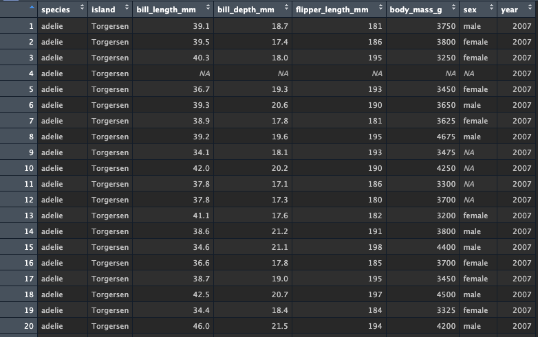
penguins %>% glimpse()
## Rows: 344
## Columns: 8
## $ species           <fct> Adelie, Adelie, Adelie, Adelie, Adelie, Adelie, Adel…
## $ island            <fct> Torgersen, Torgersen, Torgersen, Torgersen, Torgerse…
## $ bill_length_mm    <dbl> 39.1, 39.5, 40.3, NA, 36.7, 39.3, 38.9, 39.2, 34.1, …
## $ bill_depth_mm     <dbl> 18.7, 17.4, 18.0, NA, 19.3, 20.6, 17.8, 19.6, 18.1, …
## $ flipper_length_mm <int> 181, 186, 195, NA, 193, 190, 181, 195, 193, 190, 186…
## $ body_mass_g       <int> 3750, 3800, 3250, NA, 3450, 3650, 3625, 4675, 3475, …
## $ sex               <fct> male, female, female, NA, female, male, female, male…
## $ year              <int> 2007, 2007, 2007, 2007, 2007, 2007, 2007, 2007, 2007…
Notice how no argument needs to be passed to glimpse() -
the tibble penguins is piped through to the function. You
can try the same with other functions like summary() or
print(). Of course, doing this is a bit silly, since it
would be far easier to type glimpse(penguins) to get the
same result. But this should clarify the logic behind using the
pipe.
mutating within a pipe
Now lets learn the tidyverse verb mutate() and how it
can be used within a pipe. The mutate() function creates
new columns or alters existing columns. Let’s use it to simply create a
new column. The first argument for mutate() is the name of
the dataframe or tibble, and the second argument is the name of the new
variable. However, the second argument also requires a =
and then the values to set the variable to. For example
mutate(data, variable1 = 1) creates a new column named
variable1 with a value of 1 within the
dataframe data.
Let’s mutate a new variable in the penguins tibble.
First, we will create a new data set called my_penguins to
start the pipe. To do so, we start the pipe like this:
my_penguins <- penguins %>%
  mutate()
We need to put something inside mutate(). Knowing that
my_penguins is passed as the first argument to
mutate(), we can proceed directly with the new column name
and value. Let’s make a column named colour and set the
value to 'blue'
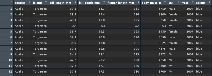
# create a new column named colour with the value 'blue'
my_penguins <- penguins %>%
  mutate(colour = 'blue')
Look at the tibble using either glimpse() or in the
viewer. You should see the new column colour has been
created at the end of the tibble, and each value has been entered as
'blue'
upgrade our mutate
Making a single value might sometimes be useful, but you might also
want to make new variables based on existing columns in the
data. This is easy with mutate, because you can place functions,
operations, and conditional statements in mutate() to
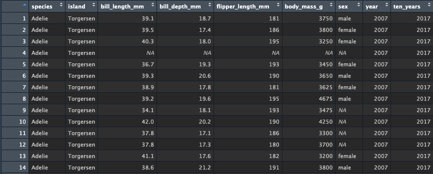
create your values. Let’s use a simple math operation to add 10 years
from each value of year. Using my_penguins, create a pipe
into mutate which creates a new column named ten_years with
the value being the result of adding 10 to the
year column. For simplicity, let’s chain
my_penguins from the original penguins data
again.
Look at the data - you should see the new column is again added to
the end of the tibble and the new values are a result of adding
10 to the years.
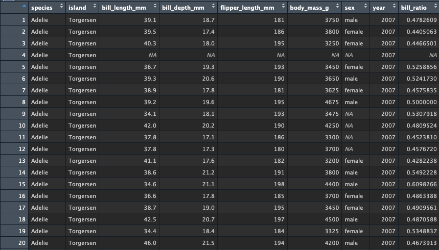
We can also do operations on multiple columns. Create a new version
of my_penguins from penguins. Then create a
pipe into a mutate call which creates a new variable
bill_ratio, which divdes bill_depth_mm by
bill_length_mm
Look at the data, yet again there is a new column added to the end of the tibble with the new values:
mutate + mutate
So far these pipes have only been piping into one more action. You
can continue the pipe by using another pipe operator after the first
action (and keep going after that). You simply add another
%>% after the second action and continue on. And, any
variable you create in the first action will become availabe in the next
action. This means you can create some intial variables, then more
variables from those created variables, and so on!
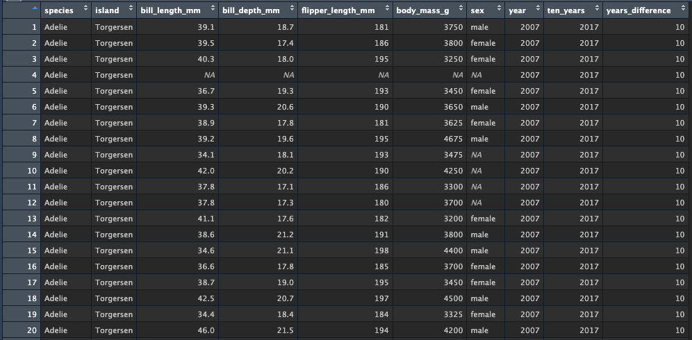
Test this out by creating yet another my_penguins tibble
from penguins. Pipe into a mutate() which
creates the ten_years variable set to
year + 10. Then, create a second pipe which goes into a
second mutate() function. The second mutate()
creates a new variable named year_difference, which is the
result of subtracting ten_years from year.
my_penguins <- penguins %>%
mutate(ten_years = year + 10) %>%
mutate(years_difference = ten_years - year)Look at the data - we see that two new variables are added at the end, and their values match with what we expect to see:
mutate x2
Actually, we don’t need to use two pipes to accomplish the same
result. This is because mutate() allows us to create more
than one variable - as many as we want actually. We simply add more
variables inside the same mutate call. The code below does the same as
above, but only uses one mutate() call:
This might not seem very amazing to you right now, but what this shows is that you can access variables as they are being created not just within the same pipe construction, but also within the same same function. This is an incredibly powerful way to create and operate on new variables very quickly.
functional mutate
We can also use existing functions in the mutate call. Lets try it
with the tolower() function, which converts text data
(i.e., string data) into all lowercase characters. Notice how the
species variable has capitalized the species of the
penguins? Lets fix that by creating a pipe into a mutate call that
overwrites species with a new column, also called
species, which is the result of calling
tolower() on species (phew…)
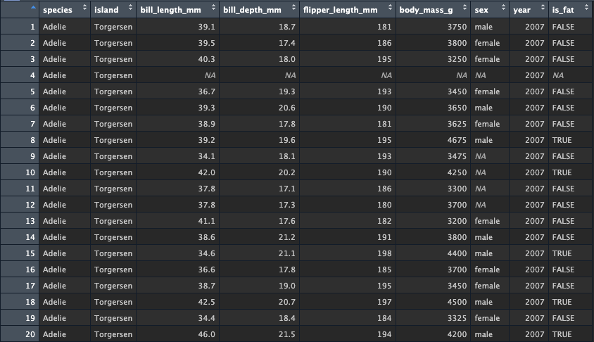
Look at the new data - note how the column is not at the end, because we overwrote the existing column. The names are also now lowercase!
functional flagging data
Another way to use mutate is to set the value of a function or
condition that performs some sort of test on the data. For example, we
could create a new column called is_fat that returns
TRUE if a penguin is over 4000 grams. We simply set the
value to be the result of the condition test for
body_mass_g > 4000
Check it out - we now have TRUE and FALSE for penguins that are below/above 4000grams.
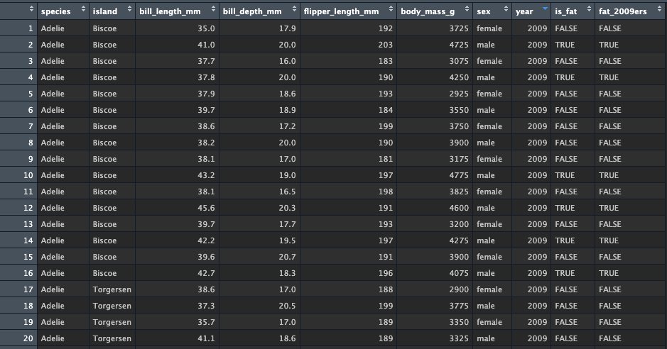
Now that you see how to create this flag, create a more complex pipe
which first uses mutate to create the is_fat variable, just
as before. Then, pipe into a new mutate function which creates the
variable fat_2009ers - this variable will check whether
is_fat is TRUE and whether
year == 2009
I use two mutate() calls below, but you could also do
this all in a single mutate call:
my_penguins <- penguins %>%
mutate(is_fat = body_mass_g > 4000) %>%
mutate(fat_2009ers = is_fat == TRUE & year == 2009)You should see something like this:
your challenge
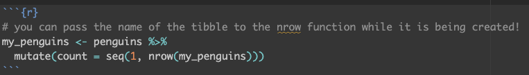
Okay, so far this has been relatively simple. Let’s challenge you to
make a variable that is a simple job: add a new variable named
count which will be a recurring list of numbers starting at
1 and ending at whatever the total number of rows a
dataframe is. Create this so that it could be applied to a tibble of
any number of rows 1 or more.
To do this, you will want to use the seq() function,
which we have already covered. We know that the starting value in
seq() should be 1, but what should the end
value be? It needs to be the total number of rows for any tibble, which
you can obtain using nrow()! So, create a
my_penguins of varying sizes which all add a
count of varying lengths!