Categorical variables in R

In this notebook we’ll take a look at how a single categorical predictor functions in a linear model. Unlike a continuous predictor, a categorical predictor defines a series of groups or categories in a variable. We can refer to the different groups or categories as different levels of a categorical predictor. In R, these need to be stored as factors.

Take the penguins data for example. There are three factor variables: species, island, and sex.

We can inspect these variables with summary() and levels()

# summary gives the counts in each level
summary(penguins$island)

##    Biscoe     Dream Torgersen 
##       168       124        52

# levels tells us the levels
levels(penguins$island)

## [1] "Biscoe"    "Dream"     "Torgersen"

summary(penguins$sex)

## female   male   NA's 
##    165    168     11

levels(penguins$sex)

## [1] "female" "male"

Using a factor as a predictor variables

We have been focusing a lot on the body mass of penguins:

ggplot(penguins, aes(x = body_mass_g)) + 
  geom_density()

## Warning: Removed 2 rows containing non-finite outside
## the scale range (`stat_density()`).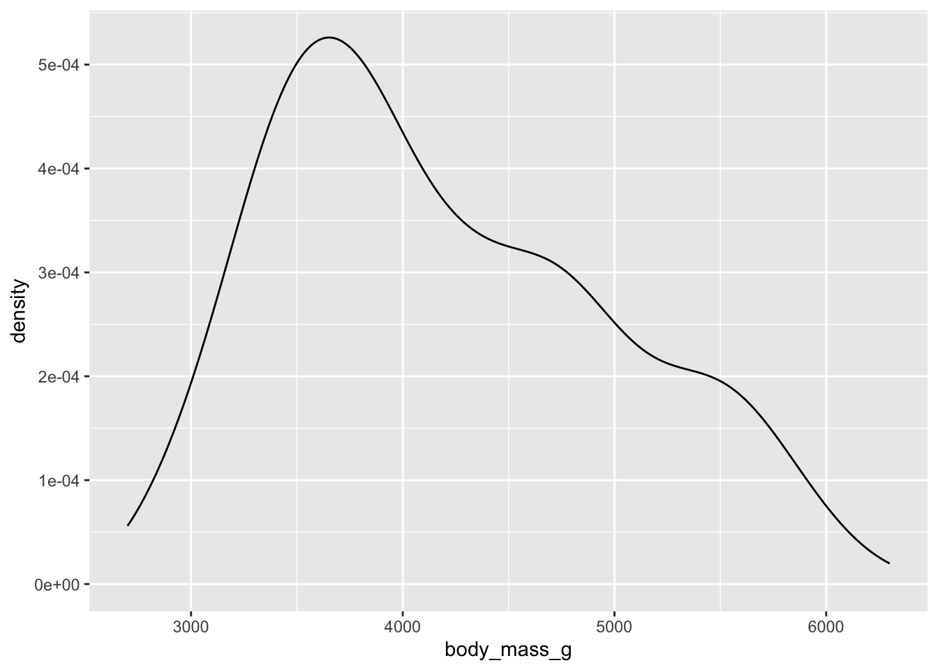

Sex and weight

We know that there is a relationship between other variables and body mass - but we haven’t yet taken and serious looks at what might be different causes of variation in penguin body mass. For example, a linear model showing that flipper length is a significant predictor of body mass doesn’t make conceptual sense - it is unlikely that flippers are determining weight of penguins.

One plausible cause is that the sex of penguins is a strong determinant of penguin body mass. Consider

# glimpse average body mass per species / sex
drop_na(penguins) %>% group_by(species, sex) %>% summarise(mean_bm = mean(body_mass_g, na.rm = T))

## `summarise()` has grouped output by 'species'.
## You can override using the `.groups` argument.

## # A tibble: 6 × 3
## # Groups:   species [3]
##   species   sex    mean_bm
##   <fct>     <fct>    <dbl>
## 1 Adelie    female   3369.
## 2 Adelie    male     4043.
## 3 Chinstrap female   3527.
## 4 Chinstrap male     3939.
## 5 Gentoo    female   4680.
## 6 Gentoo    male     5485.

# plot these raw values
ggplot(drop_na(penguins), aes(y = body_mass_g, x = sex, fill = sex)) + 
  facet_grid(. ~ species) +
  geom_violin()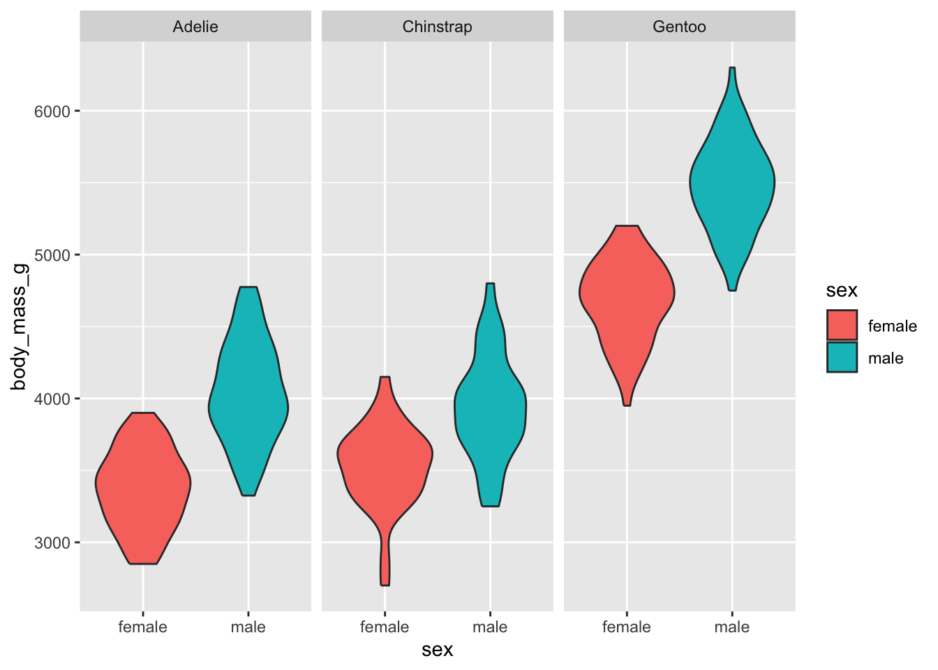

Weight and Sex

Let’s put species to the side and focus for now on sex, which only has two levels (excluding the NA values).

We want to know whether sex predicts body mass. Following our regression approach, the \(y\) variable would be body mass, and the \(x\) variable would be sex. However, sex is not a number - how can this possible work as a predictor variable?

\[ \text{body mass} \sim \text{sex} \] The answer is to convert the categorical variable into a set of numerical contrasts. The default contrast that R will apply is called dummy coding or treatment coding. This contrast sets one of the categories or levels of the variable to the value 0 and the other level to the value 1. You can see this if you use the contrasts function on the variable. Note that R will automatically place the level which is highest on alphabetical order as the reference level. The letter ‘f’ comes before ‘m’, so ‘female’ is assigned the baseline level.

# look at the default contrasts for penguin sex
contrasts(penguins$sex)

##        male
## female    0
## male      1

If female is set to 0 and male is set to 1, the linear model can now work with these levels as if they are numbers.

Let’s fit this and see what happens. Fit a linear model with sex as the predictor variable and inspect the results:

m1 <- lm(body_mass_g ~ sex, data = penguins)

What do we see in the output? It’s effectively the same as the output for a linear model with a continuous variable - we have the regression call, the distribution of the residuals, the coefficients, and information about the model fit.

What is different about this summary output is that the estimate for sex must be interpreted differently. We see there it actually says sexmale - what does that mean? It is showing us the estimate for the value of sex when it is set to male. Where did the females go? They were set as the baseline reference level, so instead of having their own coefficient, their information has been incorporated into the intercept.

summary(m1)

## 
## Call:
## lm(formula = body_mass_g ~ sex, data = penguins)
## 
## Residuals:
##     Min      1Q  Median      3Q     Max 
## -1295.7  -595.7  -237.3   737.7  1754.3 
## 
## Coefficients:
##             Estimate Std. Error t value Pr(>|t|)    
## (Intercept)  3862.27      56.83  67.963  < 2e-16 ***
## sexmale       683.41      80.01   8.542  4.9e-16 ***
## ---
## Signif. codes:  0 '***' 0.001 '**' 0.01 '*' 0.05 '.' 0.1 ' ' 1
## 
## Residual standard error: 730 on 331 degrees of freedom
##   (11 observations deleted due to missingness)
## Multiple R-squared:  0.1806, Adjusted R-squared:  0.1781 
## F-statistic: 72.96 on 1 and 331 DF,  p-value: 4.897e-16

Now, what value has the intercept taken? Where does the 3862 come from? It is simply the mean of the reference level - which is female penguins. We can verify this by quickly looking at the mean of penguins grouped by sex:

drop_na(penguins) %>% group_by(sex) %>% summarise(mean_bw = mean(body_mass_g, na.rm = T))

## # A tibble: 2 × 2
##   sex    mean_bw
##   <fct>    <dbl>
## 1 female   3862.
## 2 male     4546.

What is the value of the estimate for male penguins? It is interpreted the same as a continuous variable, a ‘one unit increase’ in sex in this case is going from 0 (female) to 1 (male). So the regression model says that going from female to male is associated with a predicted increase of 683 grams. To calculate this, we add the intercept + the estimate, which gives us 4545 grams, which is also the mean of male penguin body mass.

3862 + 683

## [1] 4545

So with treatment coding, the linear model is providing is the difference in means as the slope That’s it! The “significance” of this effect is a question as to whether the difference is meaningfully different from a difference of 0 grams. The difference, 683 grams, is divided by the standard error to get the t-statistic.

683/80

## [1] 8.5375

The resulting t-statistic is then used to obtain the p-value, the details of which we will not go into. But, for a frequentist model assuming a normal distribution, t-statistics greater than the absolute value of 1.96 will have p-values smaller than .05 and thus be considered “statistically significant”.

We can visualise the slope of the regression model by plotting the values and drawing a line connecting the means of the groups.

ggplot(drop_na(penguins), aes(y = body_mass_g, x = sex)) + 
  geom_point(alpha = .5) + 
  annotate('point', x = 1, y = 3862, color = 'blue', fill = 'blue' ,shape = 22, size = 4) + 
  annotate('point', x = 2, y = 4545, color = 'blue', fill = 'blue' ,shape = 22, size = 4) +
  annotate('segment', x = 1, xend = 2, y = 3862, yend = 4545, color = 'red', lty = 2) + 
  labs(y = 'Body Weight (grams)', x = '') + 
  jtools::theme_nice()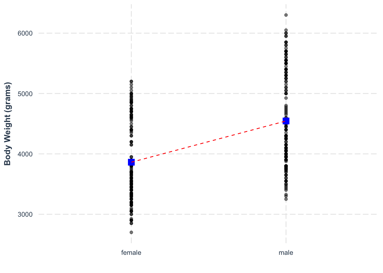

changing the reference level of a factor

Suppose we don’t want female to be the baseline and instead want male to be the baseline? We can recode the factor in R using the levels argument within the factor() function.

penguins$sex <- factor(penguins$sex, levels = c('male', 'female'))

And now the levels are swapped

levels(penguins$sex)

## [1] "male"   "female"

If we run the regression again, we can see the coefficient has changed - the effect is now a negative slope

m2 <- lm(body_mass_g ~ sex, data = penguins)

summary(m2)

## 
## Call:
## lm(formula = body_mass_g ~ sex, data = penguins)
## 
## Residuals:
##     Min      1Q  Median      3Q     Max 
## -1295.7  -595.7  -237.3   737.7  1754.3 
## 
## Coefficients:
##             Estimate Std. Error t value Pr(>|t|)    
## (Intercept)  4545.68      56.32  80.713  < 2e-16 ***
## sexfemale    -683.41      80.01  -8.542  4.9e-16 ***
## ---
## Signif. codes:  0 '***' 0.001 '**' 0.01 '*' 0.05 '.' 0.1 ' ' 1
## 
## Residual standard error: 730 on 331 degrees of freedom
##   (11 observations deleted due to missingness)
## Multiple R-squared:  0.1806, Adjusted R-squared:  0.1781 
## F-statistic: 72.96 on 1 and 331 DF,  p-value: 4.897e-16

We have simply swapped the order, so that the same line is now going down from male to female (creating a negative slope).

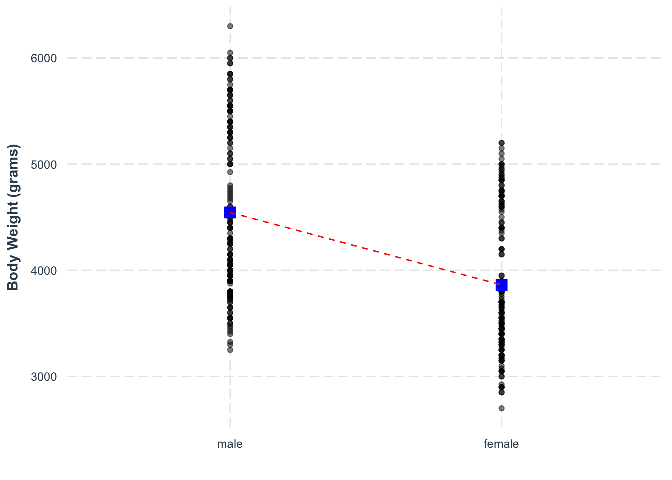
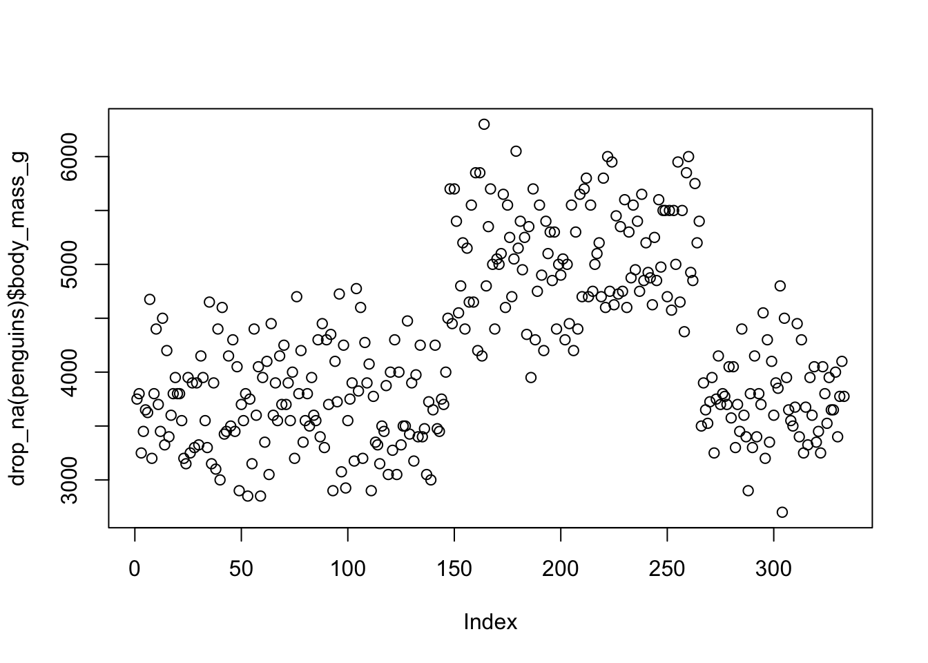
We can look at the distribution of residuals for this effect.

plot(residuals(m2))
abline(h = 0, col = 'blue')

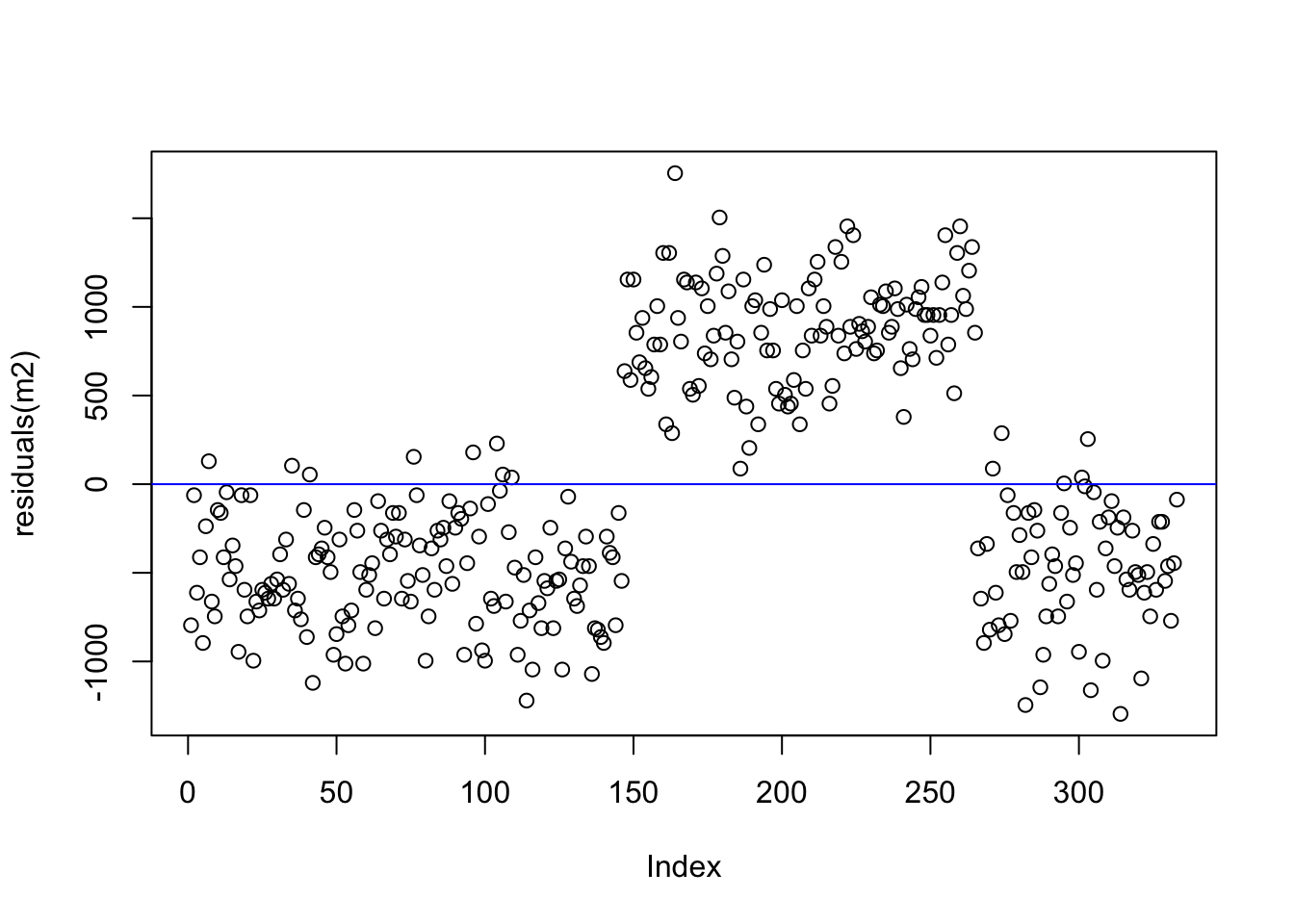
Compare to the raw data points.

plot(drop_na(penguins)$body_mass_g)

using sum contrasts

What if we don’t want either male or female to be the baseline level? Can we do that? Yes! We can apply a different contrast scheme, specifically the sum coding scheme. Sum coding will put the value of 0 in the middle of the two levels, and assign values of -1 and 1 to the two levels (these expand as we add more levels).

You can apply sum coding using the contr.sum() function, here I sum vs. treatment:

contrasts(penguins$sex)

##        female
## male        0
## female      1

Assign sum contrasts using contr.sum(). The 2 tells the function how many levels of contrasts to create:

contrasts(penguins$sex) <- contr.sum(2)

We can see that male is now 1 and female is -1:

contrasts(penguins$sex)

##        [,1]
## male      1
## female   -1

Let’s fit the linear regression and interpret the output:

m3 <- lm(body_mass_g ~ sex, data = penguins)

What has changed? We now have the coefficient sex1, which tells us the predictor has been sum coded. The intercept also shows us a value of 4204, which is neither the mean of females or males. Instead, it is the mean of their means:

summary(m3)

## 
## Call:
## lm(formula = body_mass_g ~ sex, data = penguins)
## 
## Residuals:
##     Min      1Q  Median      3Q     Max 
## -1295.7  -595.7  -237.3   737.7  1754.3 
## 
## Coefficients:
##             Estimate Std. Error t value Pr(>|t|)    
## (Intercept)   4204.0       40.0 105.088  < 2e-16 ***
## sex1           341.7       40.0   8.542  4.9e-16 ***
## ---
## Signif. codes:  0 '***' 0.001 '**' 0.01 '*' 0.05 '.' 0.1 ' ' 1
## 
## Residual standard error: 730 on 331 degrees of freedom
##   (11 observations deleted due to missingness)
## Multiple R-squared:  0.1806, Adjusted R-squared:  0.1781 
## F-statistic: 72.96 on 1 and 331 DF,  p-value: 4.897e-16

The intercept is now the mean of means:

(4545+3862)/2

## [1] 4203.5

Which is almost identical to the mean in the raw data. In this way, we can see conceptual and mathematical similarities between z-scoring and contrast sum coding.

mean(penguins$body_mass_g, na.rm = T)

## [1] 4201.754

What does the slope of 341 mean? The logic is similar. To calculate the predictors for each level, we use their underlying numeric representation, which is 1 for male and -1 for female.

So we add the intercept to the estimate which is multiplied by that numeric representation to get the predicted body weight:

\[ \text{Body Mass}_{male} = intercept + (estimate)*(1) \]

\[ \text{Body Mass}_{female} = intercept + (estimate)*(-1) \] These result in values which reflect the means of each group.

\[ \text{Body Mass}_{male} = 4204 + (341)*(1) = 4545 \]

\[ \text{Body Mass}_{male} = 4204 + (341)*(-1) = 3863 \] We can visualise this noting that it is very similar to treatment coding:

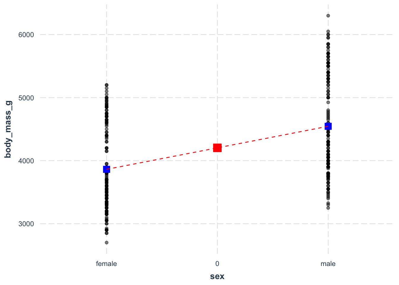
And that is a basic look into using a two-level categorical predictor in a simple linear regression.

Categorical predictors

2024-12-19