Multiple regression - two continuous \(X\)

In this notebook we extend the interpretation of linear regression to multiple regression, meaning there is more than one predictor. We will consider how adding more than one predictor to a model changes the model itself, showcasing how the model predictions change as we add new information.

To create multiple regression we simply extend the formula we already know, adding a second \(X\) predictor to our formula:

\[ \large Y \sim b_0 + (b_1*X_1) + (b_2*X_2) + \epsilon \] To predict a penguin’s body weight, we would now add the intercept to the coefficients of two variables (multipled by the observed value).

Let’s explore this with penguin body mass - we will see what a multiple regression looks like when penguin body_mass_g is predicted by two bill measurements: bill_depth_mm and bill_length_mm

First, let’s interpret two separate models, one for each \(X\) variable:

Model 1 - bill length predicting body mass

Here we see that the intercept is ~362 grams, and that for each mm in bill length, body weight increases by ~87 grams. The model indicates this is a significant effect, and that this predictor accounts for ~35% of the variance in body mass (based on the adjusted R-squared).

# bill length predicting body mass
m1 <- lm(body_mass_g ~ bill_length_mm, data = penguins)
summary(m1)

## 
## Call:
## lm(formula = body_mass_g ~ bill_length_mm, data = penguins)
## 
## Residuals:
##      Min       1Q   Median       3Q      Max 
## -1762.08  -446.98    32.59   462.31  1636.86 
## 
## Coefficients:
##                Estimate Std. Error t value            Pr(>|t|)    
## (Intercept)     362.307    283.345   1.279               0.202    
## bill_length_mm   87.415      6.402  13.654 <0.0000000000000002 ***
## ---
## Signif. codes:  0 '***' 0.001 '**' 0.01 '*' 0.05 '.' 0.1 ' ' 1
## 
## Residual standard error: 645.4 on 340 degrees of freedom
##   (2 observations deleted due to missingness)
## Multiple R-squared:  0.3542, Adjusted R-squared:  0.3523 
## F-statistic: 186.4 on 1 and 340 DF,  p-value: < 0.00000000000000022

Model 2 - bill depth predicting body mass

Here we see that the intercept is ~7488 grams, and that for each mm in bill depth, body weight decreases by ~191 grams. The model indicates this is a significant effect, and that this predictor accounts for ~22% of the variance in body mass (based on the adjusted R-squared).

# bill depth predicting body mass
m2 <- lm(body_mass_g ~ bill_depth_mm, data = penguins)
summary(m2)

## 
## Call:
## lm(formula = body_mass_g ~ bill_depth_mm, data = penguins)
## 
## Residuals:
##      Min       1Q   Median       3Q      Max 
## -1607.38  -510.10   -66.96   462.43  1819.28 
## 
## Coefficients:
##               Estimate Std. Error t value            Pr(>|t|)    
## (Intercept)    7488.65     335.22   22.34 <0.0000000000000002 ***
## bill_depth_mm  -191.64      19.42   -9.87 <0.0000000000000002 ***
## ---
## Signif. codes:  0 '***' 0.001 '**' 0.01 '*' 0.05 '.' 0.1 ' ' 1
## 
## Residual standard error: 708.1 on 340 degrees of freedom
##   (2 observations deleted due to missingness)
## Multiple R-squared:  0.2227, Adjusted R-squared:  0.2204 
## F-statistic: 97.41 on 1 and 340 DF,  p-value: < 0.00000000000000022

Model 3 - bill length and bill depth predicting body mass

Now fit a model with both \(X\) in the model. What is different?

The intercept is now 3343 grams. Remember that this is the predicted value of body weight when all \(X\) are held at 0.
for each increase in bill length, body mass increases by 75 grams. This is a decreased effect of about 12 grams from the estimate of m1
for each increase in bill depth, body mass decreases by 142 grams. This is a decreased effect of about 50 grams from m2
this model now explains ~47% of the variance in body mass, an increase of about 12% from m1 and about 25% from m2

# bill length and bill depth predicting body mass
m3 <- lm(body_mass_g ~ bill_length_mm + bill_depth_mm, data = penguins )
summary(m3)

## 
## Call:
## lm(formula = body_mass_g ~ bill_length_mm + bill_depth_mm, data = penguins)
## 
## Residuals:
##      Min       1Q   Median       3Q      Max 
## -1804.61  -454.83     8.15   463.53  1544.82 
## 
## Coefficients:
##                Estimate Std. Error t value             Pr(>|t|)    
## (Intercept)    3343.136    429.912   7.776   0.0000000000000905 ***
## bill_length_mm   75.281      5.971  12.608 < 0.0000000000000002 ***
## bill_depth_mm  -142.723     16.507  -8.646 < 0.0000000000000002 ***
## ---
## Signif. codes:  0 '***' 0.001 '**' 0.01 '*' 0.05 '.' 0.1 ' ' 1
## 
## Residual standard error: 585.1 on 339 degrees of freedom
##   (2 observations deleted due to missingness)
## Multiple R-squared:  0.4708, Adjusted R-squared:  0.4677 
## F-statistic: 150.8 on 2 and 339 DF,  p-value: < 0.00000000000000022

What is the predicted body mass of a penguin with a bill length of 40mm and a bill depth of 18mm?

First consider the values we need to enter:

\[ \text{Body Mass} = \text{Intercept} + (75.281 * \text{Bill Length}) + (-142.723 * \text{Bill Depth}) \]

Calculate the values multiplied by their coefficients

\[ \text{Body Mass} = 3343.136 + (75.281 * 40) + (-142.723 * 18) \] Then finish summing the results

\[ \text{Body Mass} = 3343.136 + 3011.24 + -2569.014 \ \] The final predicted body weight is ~3785 grams.

\[ \text{Body Mass} = 3785.362 \ \]

\(X1\) controlling for \(X2\) (and vice versa)

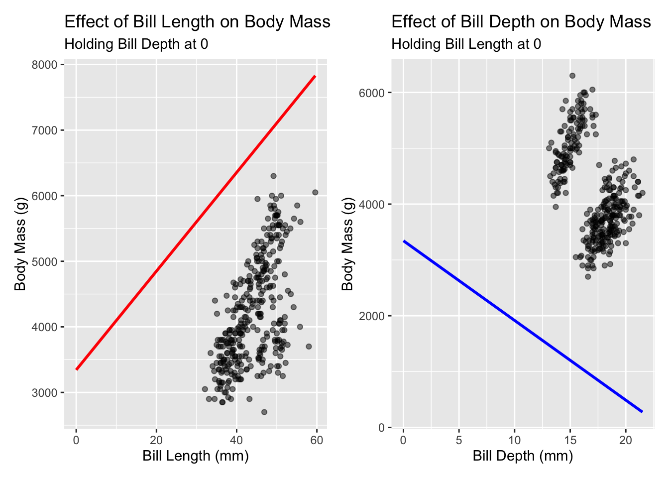
What we have done with our new model is asked for it to tell us the effects of bill_length_mm or bill_depth_mm when controlling for the value of either other variable. It is controlled in the sense that the intercept reflects the \(Y\) when both variables are held at 0 - which means “none of that thing.”

is 0 a meaningful value?

Let’s visualise these effects independently, which will serve as a reminder why holding something at 0 may not be very meaningful:

using centered data

Let’s fit the exact same model, but this time with centered values

# I will use scale() to center the values
penguins$bill_length_mm_c <- scale(penguins$bill_length_mm, scale = F, center = T)
penguins$bill_depth_mm_c <- scale(penguins$bill_depth_mm, scale = F, center = T)

m4 <- lm(body_mass_g ~ bill_length_mm_c + bill_depth_mm_c, data = penguins)

What changes?

summary(m4)

## 
## Call:
## lm(formula = body_mass_g ~ bill_length_mm_c + bill_depth_mm_c, 
##     data = penguins)
## 
## Residuals:
##      Min       1Q   Median       3Q      Max 
## -1804.61  -454.83     8.15   463.53  1544.82 
## 
## Coefficients:
##                  Estimate Std. Error t value            Pr(>|t|)    
## (Intercept)      4201.754     31.638 132.809 <0.0000000000000002 ***
## bill_length_mm_c   75.281      5.971  12.608 <0.0000000000000002 ***
## bill_depth_mm_c  -142.723     16.507  -8.646 <0.0000000000000002 ***
## ---
## Signif. codes:  0 '***' 0.001 '**' 0.01 '*' 0.05 '.' 0.1 ' ' 1
## 
## Residual standard error: 585.1 on 339 degrees of freedom
##   (2 observations deleted due to missingness)
## Multiple R-squared:  0.4708, Adjusted R-squared:  0.4677 
## F-statistic: 150.8 on 2 and 339 DF,  p-value: < 0.00000000000000022

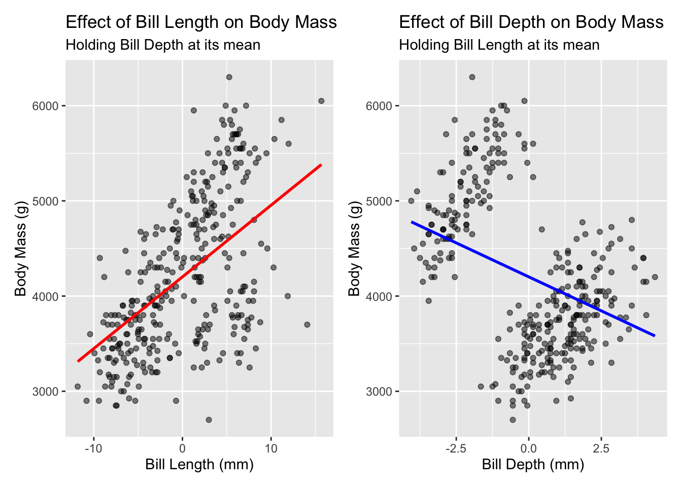
But when we plot the new predicted values, we now have a meaningful range with values that make sense.

Question - which predictor has the strongest effect? How do you know?

including z-scores

Let’s consider a z-scored version. Question - which predictor has the strongest effect? How do you know?

# fit a z-scored model
penguins$bill_length_mm_z <- scale(penguins$bill_length_mm, scale = T, center = T)
penguins$bill_depth_mm_z <- scale(penguins$bill_depth_mm, scale = T, center = T)

m5 <- lm(body_mass_g ~ bill_length_mm_z + bill_depth_mm_z, data = penguins)
summary(m5)

## 
## Call:
## lm(formula = body_mass_g ~ bill_length_mm_z + bill_depth_mm_z, 
##     data = penguins)
## 
## Residuals:
##      Min       1Q   Median       3Q      Max 
## -1804.61  -454.83     8.15   463.53  1544.82 
## 
## Coefficients:
##                  Estimate Std. Error t value            Pr(>|t|)    
## (Intercept)       4201.75      31.64 132.809 <0.0000000000000002 ***
## bill_length_mm_z   411.00      32.60  12.608 <0.0000000000000002 ***
## bill_depth_mm_z   -281.85      32.60  -8.646 <0.0000000000000002 ***
## ---
## Signif. codes:  0 '***' 0.001 '**' 0.01 '*' 0.05 '.' 0.1 ' ' 1
## 
## Residual standard error: 585.1 on 339 degrees of freedom
##   (2 observations deleted due to missingness)
## Multiple R-squared:  0.4708, Adjusted R-squared:  0.4677 
## F-statistic: 150.8 on 2 and 339 DF,  p-value: < 0.00000000000000022

The answer is in that even though bill_depth and bill_length are both measured on the same unit, they have different underlying distributions. The length has a longer overall range, with a different standard deviation

mean(penguins$bill_length_mm, na.rm = T)

## [1] 43.92193

sd(pengui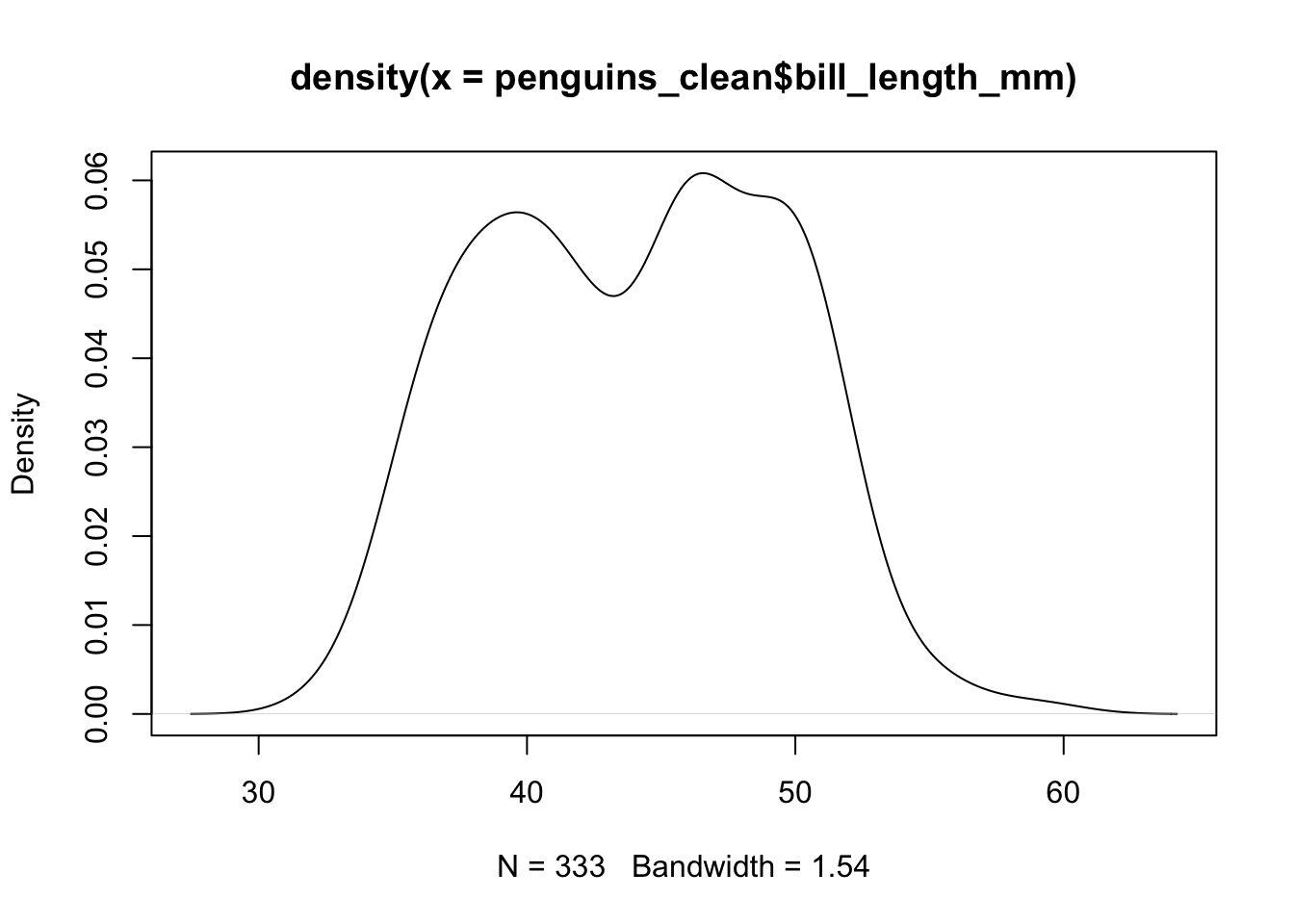ns$bill_length_mm, na.rm = T)

## [1] 5.459584

plot(density(penguins_clean$bill_length_mm))

mean(penguins$bill_depth_mm, na.rm = T)

## [1] 17.15117

sd(pengui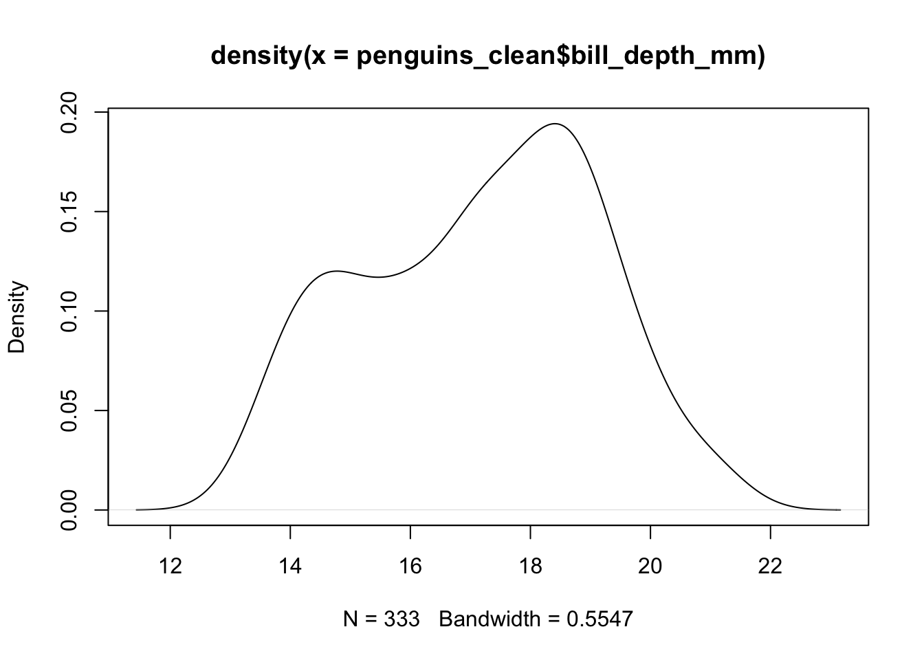ns$bill_depth_mm, na.rm = T)

## [1] 1.974793

plot(density(penguins_clean$bill_depth_mm))

plotting z-score simple effects

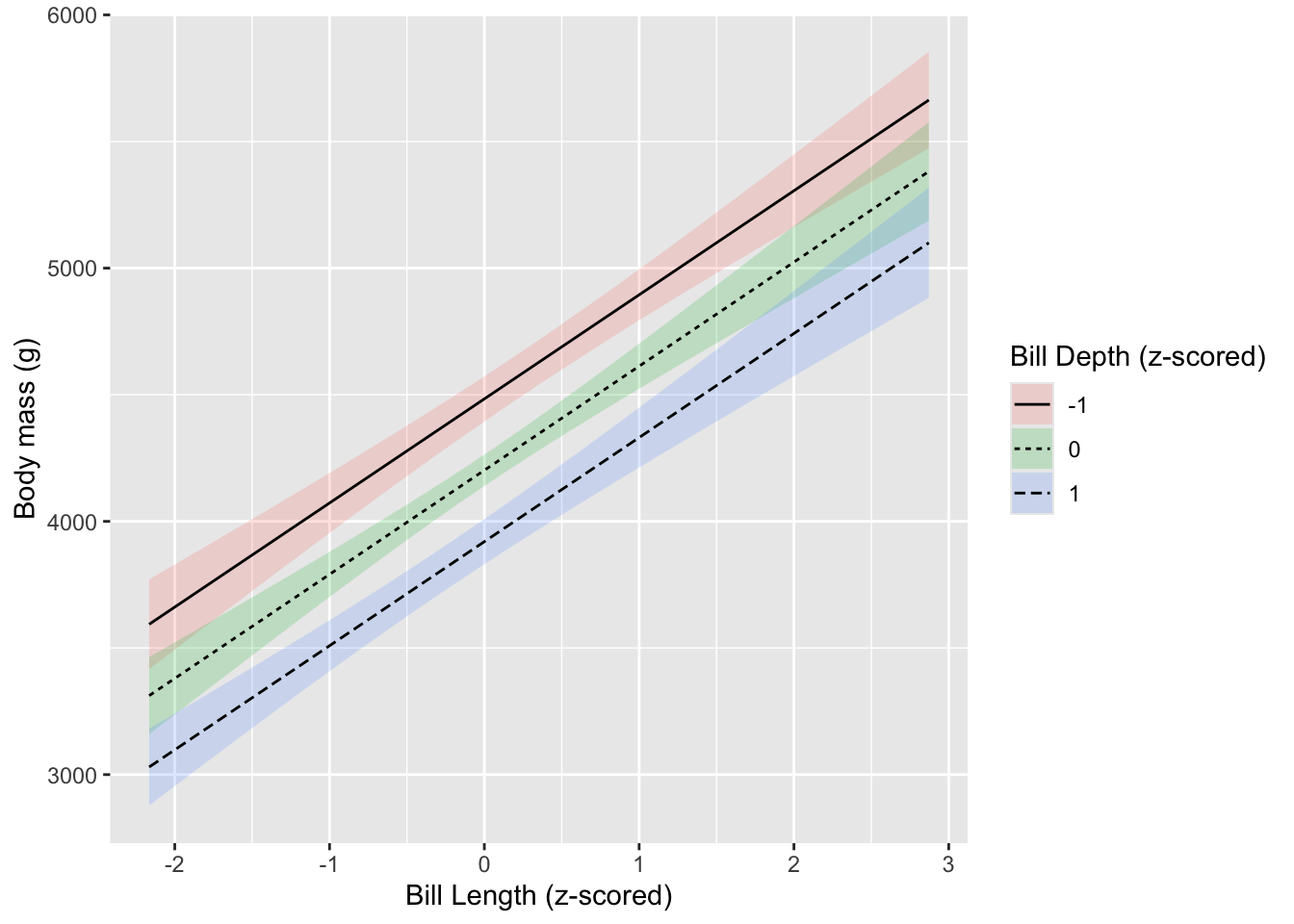
Since we have converted our variables into z-scored, we can start looking at the effects of one variable while controlling for the effects of another variable at specific points! For instance, we could choose to look at the effects of Bill Length at the mean as well as +/- 1 standard deviation of Bill Depth!

We can look at the other way too…

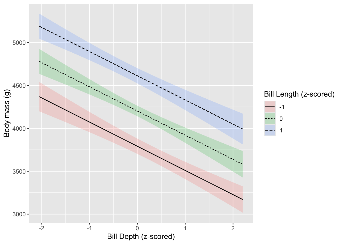
Giving the plots different values of either \(X\) changes the intercept, but it does not change the slope - the overall degree of the angle or effect. To do that, we would need to look at the interaction between the two variables.

multiple regression

2024-11-20