filtering data
2025-04-10
This is the first notebook using functions from the popular
tidyverse set of packages. In this notebook, we explore a
fundamental data structure, the tibble/dataframe, and learn how to
perform basic filtering functions on the data using conditional
tests.
What is tidyverse?
the tidyverse is a set of R packages combined into a
single library/package. The packages are intended to do various
data-related things, such as manipulating and shaping data, visualizing
data, and more. In this notebook we will look at some of the basic
functions related to data filtering and querying.
The first thing to do is to install the package, which you can do
using install.packages('tidyverse'). Once you’ve installed
it, go ahead and load it using library()
You’ll notice that the output says it is attaching the core tidyverse packages, highlighting that this is actually an ecosystem of different packages.
Making some penguins
Lets use the penguins data set which is included in the
palmerpenguins package. Load the package first (and install
it if necessary)
Once loaded, we have access to the penguins data set,
which we can view by simply typing its name.
## # A tibble: 333 × 9
##    species island    bill_length_mm bill_depth_mm flipper_length_mm body_mass_g
##    <fct>   <fct>              <dbl>         <dbl>             <int>       <int>
##  1 Adelie  Torgersen           39.1          18.7               181        3750
##  2 Adelie  Torgersen           39.5          17.4               186        3800
##  3 Adelie  Torgersen           40.3          18                 195        3250
##  4 Adelie  Torgersen           36.7          19.3               193        3450
##  5 Adelie  Torgersen           39.3          20.6               190        3650
##  6 Adelie  Torgersen           38.9          17.8               181        3625
##  7 Adelie  Torgersen           39.2          19.6               195        4675
##  8 Adelie  Torgersen           41.1          17.6               182        3200
##  9 Adelie  Torgersen           38.6          21.2               191        3800
## 10 Adelie  Torgersen           34.6          21.1               198        4400
## # ℹ 323 more rows
## # ℹ 3 more variables: sex <fct>, year <int>, flipper_length_mm_z <dbl>
Let’s actually add the penguins data set to our global
environment, using the data() function:
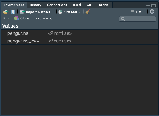
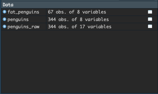
Viewing the dataframe in the global environment
Take a look at your global environment, you might see something like this:
Just click onto the name of penguins and you should see the “promise” turn into the actual data object, like this:
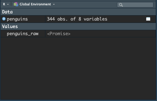
Now we have access to the penguins dataframe, which is a
data format we will use heavily. Technically, this dataframe is in the
form of a tibble, which is a type of dataframe preferred by
tidyverse.
Click the blue arrow to get a glimpse of the structure of the tibble:
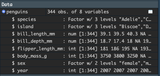
There is a rich amount of information here:
- there are 344 obs (observations) in the data
- there are 8 variables (i.e., columns)
- the names of the variables are
species,island,bill_length_mm,bill_depth_mm,flipper_length_mm,body_mass_g,sex, andyear - the variables are of different types:
Factor,num, orint.
We will discuss the differences among these variables as we go. The point here is that we can quickly get an overview of the tibble simply by looking at it in the global environment pane.
We can use the glimpse() function to get the same
information in R itself:
## Rows: 344
## Columns: 8
## $ species           <fct> Adelie, Adelie, Adelie, Adelie, Adelie, Adelie, Adel…
## $ island            <fct> Torgersen, Torgersen, Torgersen, Torgersen, Torgerse…
## $ bill_length_mm    <dbl> 39.1, 39.5, 40.3, NA, 36.7, 39.3, 38.9, 39.2, 34.1, …
## $ bill_depth_mm     <dbl> 18.7, 17.4, 18.0, NA, 19.3, 20.6, 17.8, 19.6, 18.1, …
## $ flipper_length_mm <int> 181, 186, 195, NA, 193, 190, 181, 195, 193, 190, 186…
## $ body_mass_g       <int> 3750, 3800, 3250, NA, 3450, 3650, 3625, 4675, 3475, …
## $ sex               <fct> male, female, female, NA, female, male, female, male…
## $ year              <int> 2007, 2007, 2007, 2007, 2007, 2007, 2007, 2007, 2007…
We can also ask for basic information about the variables in the data
using summary(). Try it out - here we can see some
statistical information about the distribution of each of the
variables.
##       species          island    bill_length_mm  bill_depth_mm
##  Adelie   :152   Biscoe   :168   Min.   :32.10   Min.   :13.10
##  Chinstrap: 68   Dream    :124   1st Qu.:39.23   1st Qu.:15.60
##  Gentoo   :124   Torgersen: 52   Median :44.45   Median :17.30
##                                  Mean   :43.92   Mean   :17.15
##                                  3rd Qu.:48.50   3rd Qu.:18.70
##                                  Max.   :59.60   Max.   :21.50
##                                  NA's   :2       NA's   :2
##  flipper_length_mm  body_mass_g       sex           year
##  Min.   :172.0     Min.   :2700   female:165   Min.   :2007
##  1st Qu.:190.0     1st Qu.:3550   male  :168   1st Qu.:2007
##  Median :197.0     Median :4050   NA's  : 11   Median :2008
##  Mean   :200.9     Mean   :4202                Mean   :2008
##  3rd Qu.:213.0     3rd Qu.:4750                3rd Qu.:2009
##  Max.   :231.0     Max.   :6300                Max.   :2009
##  NA's   :2         NA's   :2
Viewing the entire dataframe in the interactive viewer
Now, try clicking on penguins in the Global Environment (click the
name penguins). This should open up a new tab in R Studio
which shows you the entirety of the data, like this:
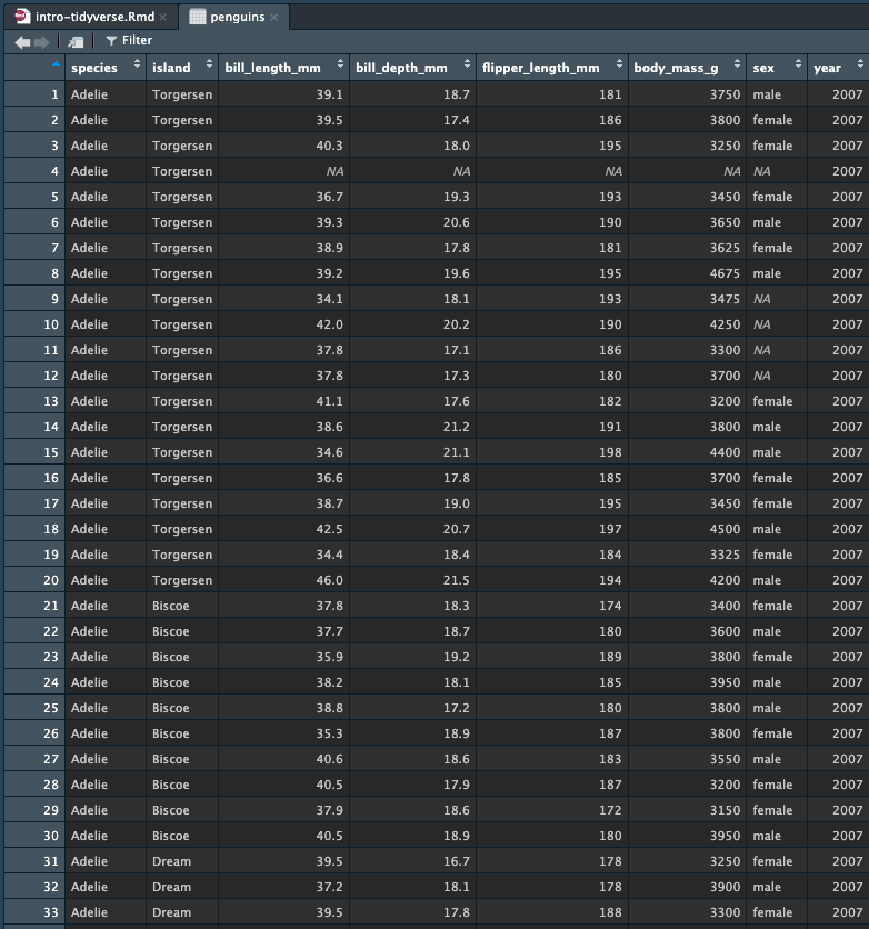
This view allows you to scan the entire data set. You can also sort and filter in the view. You cannot do any modifications to the data in this view.
long vs. wide structure
The data in penguins is organised using the long data
format. This means that each row is a single observation. In this case,
each row is a different penguin. The columns are the different variables
and measurements for each observation. So we can see that the first
penguin is male from 2007 and has a body mass of 3750 grams.
The alternative format is wide format, where each column is an observation and the rows are different variables. Programs like SPSS use such organisations. However, almost everything we do with R and our analyses will expect data to be in long format - so get used to it!
tidyverse verbs - filter()
There are some very useful functions or verbs that we can use in tidyverse to make sense of the data. For example, say we want to count the number of penguins born in a certain year, or only include penguins of a certain body mass or flipper width. This sort of data wrangling is fundamental to data science and statistics, and helps us tell different stories about out data.
Let’s start with filter(). The filter()
function will apply a conditional argument to a specified
column in a dataframe/tibble. It will do this test for each row
in the data.
Conditional arguments are written using symbols such as
==, <, >. See below for a
list:
== |
equals to |
!= |
does not equal |
< |
less than |
<= |
less than or equal to |
> |
greater than |
>= |
greater than or equal to |
With these tests, we can ask R to give us more specific information from our data. For example, let’s ask for all of the penguins which have a body mass of 5000 grams or more.
filter on body mass
To use filter(), we first provide the data we want to
filter, and then the test we want to perform. The test needs to be
conducted on a column in the data. In this case, we are interested in
body_mass_g. We want all penguins which weight more than
this, so our condition test will be
body_mass_g >= 5000:
## # A tibble: 67 × 8
##    species island bill_length_mm bill_depth_mm flipper_length_mm body_mass_g
##    <fct>   <fct>           <dbl>         <dbl>             <int>       <int>
##  1 Gentoo  Biscoe           50            16.3               230        5700
##  2 Gentoo  Biscoe           50            15.2               218        5700
##  3 Gentoo  Biscoe           47.6          14.5               215        5400
##  4 Gentoo  Biscoe           46.7          15.3               219        5200
##  5 Gentoo  Biscoe           46.8          15.4               215        5150
##  6 Gentoo  Biscoe           49            16.1               216        5550
##  7 Gentoo  Biscoe           48.4          14.6               213        5850
##  8 Gentoo  Biscoe           49.3          15.7               217        5850
##  9 Gentoo  Biscoe           49.2          15.2               221        6300
## 10 Gentoo  Biscoe           48.7          15.1               222        5350
## # ℹ 57 more rows
## # ℹ 2 more variables: sex <fct>, year <int>
Voila, if we look at the output, we can see that the tibble is 67 x 8, meaning 67 rows or 67 observations - which means 67 penguins weigh 5000 grams or more. Since the total number of penguins is 344, this means most penguins seem to weigh under 5000 grams.
It is not very useful to have the output only exist in the console,
we may instead prefer to save the results of these tests to new
variables. Let’s create a tibble named fat_penguins which
includes only penguins which weigh over 5000 grams.
A new tibble has been added to the global environment, which has the name we gave it. You can now operate on this new tibble in much the same way as we did on penguins, and you can also open it up in the viewer to look at these penguins.
filter on sex
Let’s do another filter, this time using a variable stored as text
data. We will create a new tibble called fat_boy_penguins
which includes all the fat penguins who are male. The conditional test
will thus be on the column sex, and we want all the rows
where sex is equal to the value male. The test
is thus typed like this: sex == 'male'. Note that we use
double equal signs, and we must encase the value male
within quotes (representing the text data).
Oh my - we see that of the 67 fat penguins, 59 of them are male penguins. Is there a potential relationship between sex and body size in this penguin domain?!
Look at the data - do you notice anything else? For example, in the Species column?
filter sex and body mass in one line
We can do more than one test within the same filter command. For
example, instead of two separate steps, let’s filter the
penguins data to return all male penguins who are over 5000
grams in a single command. To do so, we can create a more complex
conditional statement by joining two conditions together with the
& operator, meaning and. So we want all
penguins who are male and are also 5000 grams or more. The condition
will be on two columns, like this:
sex == 'male' & body_mass_g >= 5000
Here is the command, although I do not save this to a variable.
## # A tibble: 59 × 8
##    species island bill_length_mm bill_depth_mm flipper_length_mm body_mass_g
##    <fct>   <fct>           <dbl>         <dbl>             <int>       <int>
##  1 Gentoo  Biscoe           50            16.3               230        5700
##  2 Gentoo  Biscoe           50            15.2               218        5700
##  3 Gentoo  Biscoe           47.6          14.5               215        5400
##  4 Gentoo  Biscoe           46.7          15.3               219        5200
##  5 Gentoo  Biscoe           46.8          15.4               215        5150
##  6 Gentoo  Biscoe           49            16.1               216        5550
##  7 Gentoo  Biscoe           48.4          14.6               213        5850
##  8 Gentoo  Biscoe           49.3          15.7               217        5850
##  9 Gentoo  Biscoe           49.2          15.2               221        6300
## 10 Gentoo  Biscoe           48.7          15.1               222        5350
## # ℹ 49 more rows
## # ℹ 2 more variables: sex <fct>, year <int>
Your turn!
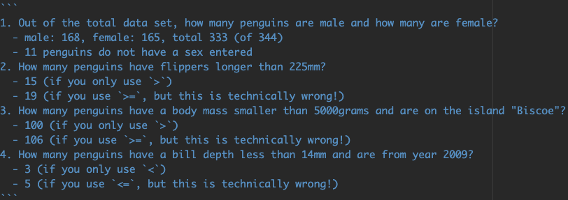
Play around with filter to answer the following questions:
- Out of the total data set, how many penguins are male and how many are female? (Bonus question, why does the total not add up to 344?)
- How many penguins have flippers longer than 225mm?
- How many penguins have a body mass smaller than 5000grams and are on the island “Biscoe”?
- How many penguins have a bill depth less than 14mm and are from year 2009?