categorical by continuous interaction
2025-08-14
Multiple regression - one continuous and one categorical \(X\) in an interaction
In this lesson we continue looking at interactions between two predictor variables. This time, between a continuous and categorical \(x\). We have already learned the formula for an interaction:
\[ \large Y \sim b_0 + (b_1*X_1) + (b_2*X_2) + b_3 * (X_1 * X_2) + \epsilon \]
And we have already learned how a categorical variable is “converted” into numbers in order to fit within a regression formula.
So it is a matter of applying those bits of knowledge to the interaction terms.
# load in the data
library(tidyverse)
library(palmerpenguins)
data(penguins)
penguins <- drop_na(penguins)
Flippers and sex
In this lesson, we will consider an interaction between penguin flipper length and penguin sex, and how this may (or may not) provide us with more information about a penguin’s body weight.
Let’s first remind ourselves whether these variables have an effect on their own. Looking at this plot, is there a relationship between flipper length and body mass?
ggplot(penguins, aes(x = flipper_length_mm, y = body_mass_g)) +
  geom_point() +
  jtools::theme_nice() +
  labs(title = 'Effect of flipper length on body mass')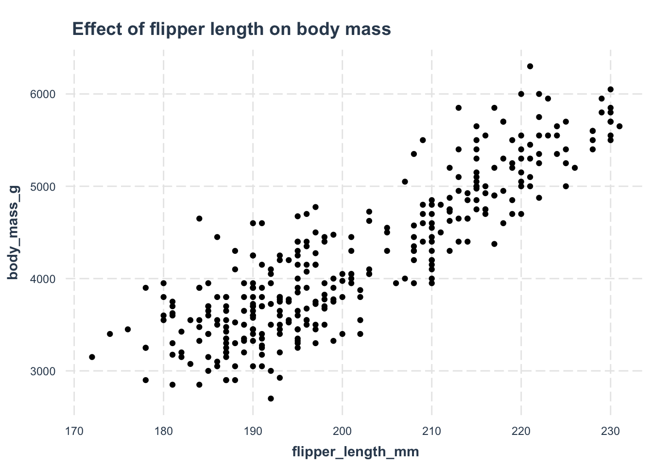
We can test this with a single predictor lm:
# center flipper length
penguins$flipper_length_mm_c <- penguins$flipper_length_mm - mean(penguins$flipper_length_mm)
# can you interpret the intercept and effect?
m1 <- lm(body_mass_g ~ flipper_length_mm_c, data = penguins)
summary(m1)##
## Call:
## lm(formula = body_mass_g ~ flipper_length_mm_c, data = penguins)
##
## Residuals:
## Min 1Q Median 3Q Max
## -1057.33 -259.79 -12.24 242.97 1293.89
##
## Coefficients:
## Estimate Std. Error t value Pr(>|t|)
## (Intercept) 4207.06 21.55 195.18 <2e-16 ***
## flipper_length_mm_c 50.15 1.54 32.56 <2e-16 ***
## ---
## Signif. codes: 0 '***' 0.001 '**' 0.01 '*' 0.05 '.' 0.1 ' ' 1
##
## Residual standard error: 393.3 on 331 degrees of freedom
## Multiple R-squared: 0.7621, Adjusted R-squared: 0.7614
## F-statistic: 1060 on 1 and 331 DF, p-value: < 2.2e-16Now, what about sex?
ggplot(penguins, aes(x = sex, y = body_mass_g)) +
 # facet_grid(. ~ sex) +
  geom_point() +
  jtools::theme_nice()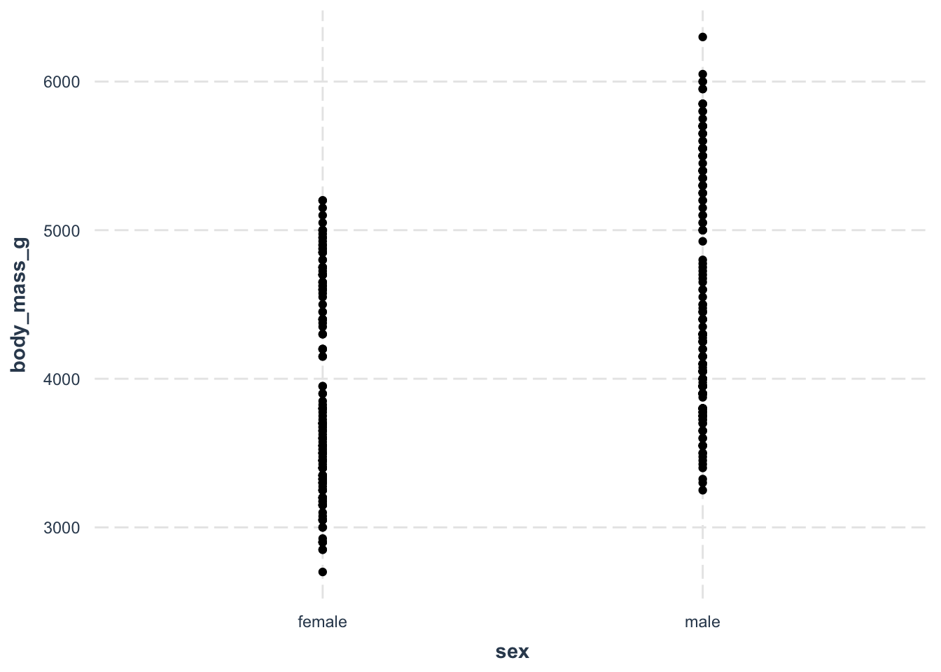
# can you interpret the intercept and effect?
m2 <- lm(body_mass_g ~ sex, data = penguins)
summary(m2)
##
## Call:
## lm(formula = body_mass_g ~ sex, data = penguins)
##
## Residuals:
## Min 1Q Median 3Q Max
## -1295.7 -595.7 -237.3 737.7 1754.3
##
## Coefficients:
## Estimate Std. Error t value Pr(>|t|)
## (Intercept) 3862.27 56.83 67.963 < 2e-16 ***
## sexmale 683.41 80.01 8.542 4.9e-16 ***
## ---
## Signif. codes: 0 '***' 0.001 '**' 0.01 '*' 0.05 '.' 0.1 ' ' 1
##
## Residual standard error: 730 on 331 degrees of freedom
## Multiple R-squared: 0.1806, Adjusted R-squared: 0.1781
## F-statistic: 72.96 on 1 and 331 DF, p-value: 4.897e-16But what about their interaction?
Looking at this plot, we see that the general pattern of flipper length does not really change between female and male penguins. In both cases, longer flippers are associated with heavier penguins. But we can still test this as an interaction!
ggplot(penguins, aes(x = flipper_length_mm, y = body_mass_g)) +
  facet_grid(. ~ sex) +
  geom_point() +
  jtools::theme_nice() +
  labs(title = 'Does sex moderate flippper length?')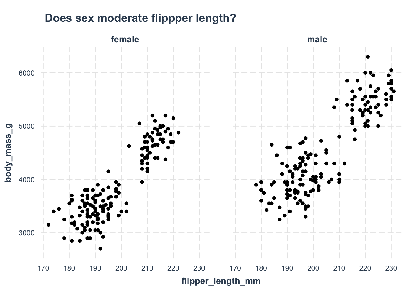
fit the interaction model
How do we interpet this?
sexmaleis the difference between male and female penguins when flipper length is held at its mean
flipper_length_mm_cis the effect of flipper length whensexis set to 0. Because this is dummy-coded, that means it is the effect of flipper length on body weight for female penguinssexmale:flipper_length_mm_cis the difference in the effect of flipper length between males and females. The difference in the slope is very small, effectively zero.
# do you know how to interpret the model?
m3 <- lm(body_mass_g ~ sex*flipper_length_mm_c, data = penguins)
summary(m3)
##
## Call:
## lm(formula = body_mass_g ~ sex * flipper_length_mm_c, data = penguins)
##
## Residuals:
## Min 1Q Median 3Q Max
## -909.36 -246.58 -3.13 237.18 1065.19
##
## Coefficients:
## Estimate Std. Error t value Pr(>|t|)
## (Intercept) 4032.1796 28.8836 139.601 < 2e-16 ***
## sexmale 347.6734 40.4404 8.597 3.37e-16 ***
## flipper_length_mm_c 47.1527 2.2264 21.179 < 2e-16 ***
## sexmale:flipper_length_mm_c -0.2942 2.9242 -0.101 0.92
## ---
## Signif. codes: 0 '***' 0.001 '**' 0.01 '*' 0.05 '.' 0.1 ' ' 1
##
## Residual standard error: 356.4 on 329 degrees of freedom
## Multiple R-squared: 0.8058, Adjusted R-squared: 0.8041
## F-statistic: 455.2 on 3 and 329 DF, p-value: < 2.2e-16Like the continuous by continuous interaction, we are still dealing with conditional means. But in this case, we only have two possible values for the categorical variable: male or female penguins. So the possible condition are much fewer when compared to two continuous variables.
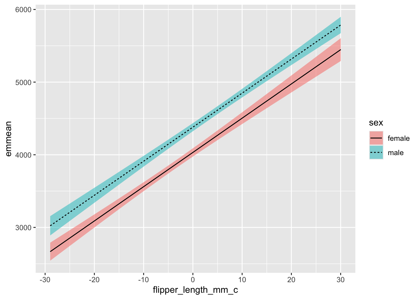
Let’s plot the two slopes to see how much they differ: almost imperceptible. Now how the model still captures the relative difference in body weight between male and female penguins, in that the male predicted weight is always higher than the female. But the effect of flipper length is almost the same, regardless of sex. There is no significant interaction between them.
doing the same with sum coding
Here is a model with sum coding applied.
flipper_length_mm_cis the effect of flipper length across both males and females, the average effectsex1is the effect of sex while flipper length is held at its mean. Recall that female will be 1, and males -1, and these are the values the term uses. So males are 173 grams above the mean body weight when flipper length is held at its mean.flipper_length_mm_c:sex1is the interaction term again, and shows us how much the slope differs between males and females. This time, it shows us how much the effect of flipper length affects the deviation of either group from their grand mean (in dummy coding, this was the straight-up difference between the two groups).
##        [,1]
## female    1
## male -1##
## Call:
## lm(formula = body_mass_g ~ flipper_length_mm_c * sex, data = penguins)
##
## Residuals:
## Min 1Q Median 3Q Max
## -909.36 -246.58 -3.13 237.18 1065.19
##
## Coefficients:
## Estimate Std. Error t value Pr(>|t|)
## (Intercept) 4206.0163 20.2202 208.010 < 2e-16 ***
## flipper_length_mm_c 47.0056 1.4621 32.149 < 2e-16 ***
## sex1 -173.8367 20.2202 -8.597 3.37e-16 ***
## flipper_length_mm_c:sex1 0.1471 1.4621 0.101 0.92
## ---
## Signif. codes: 0 '***' 0.001 '**' 0.01 '*' 0.05 '.' 0.1 ' ' 1
##
## Residual standard error: 356.4 on 329 degrees of freedom
## Multiple R-squared: 0.8058, Adjusted R-squared: 0.8041
## F-statistic: 455.2 on 3 and 329 DF, p-value: < 2.2e-16Even though we did deviation coding, the magnitude of the effect doesn’t change in the visualisation…
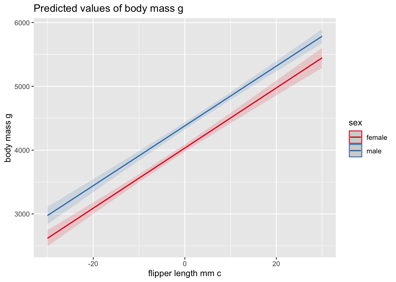
none of the continuous predictors interact significantly with sex
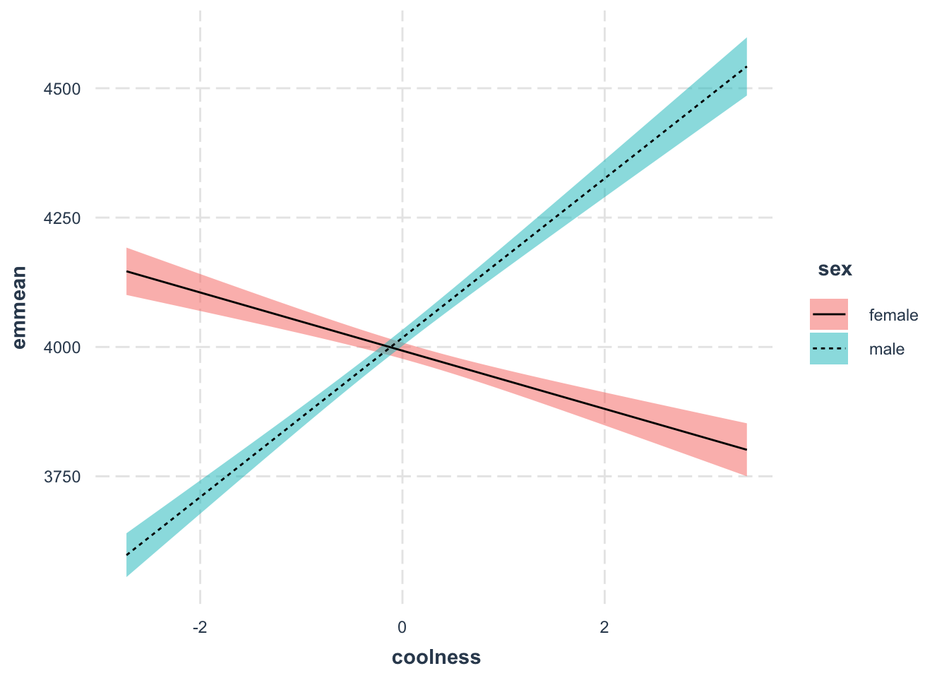
That sucks. I can’t show you an example of a significant continuous by categorical interaction in this data. Unless I make up some data.
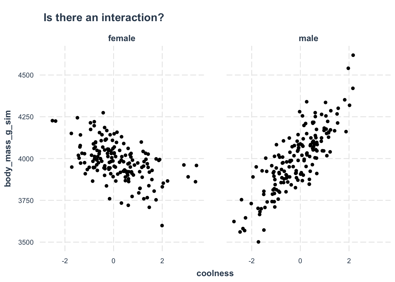
Model the interaction - can you interpret this? coolness has been centered.
##
## Call:
## lm(formula = body_mass_g_sim ~ sex * coolness, data = penguins)
##
## Residuals:
##      Min       1Q   Median       3Q      Max
## -281.664  -67.511   -4.655   68.296  282.222
##
## Coefficients:
##               Estimate Std. Error t value Pr(>|t|)
## (Intercept)   4005.280      5.641 710.092   <2e-16 ***
## sex1           -12.501      5.641  -2.216   0.0274 *
## coolness        48.860      5.428   9.002   <2e-16 ***
## sex1:coolness -105.097      5.428 -19.362   <2e-16 ***
## ---
## Signif. codes:  0 '***' 0.001 '**' 0.01 '*' 0.05 '.' 0.1 ' ' 1
##
## Residual standard error: 101.9 on 329 degrees of freedom
## Multiple R-squared:  0.578,  Adjusted R-squared:  0.5742
## F-statistic: 150.2 on 3 and 329 DF,  p-value: < 2.2e-16
Plot the interaction -
