Multiple regression - two continuous \(X\) in an interaction

We have recently looked at how including more than one continuous variable in a regression model works to “control” for the other variables. This means that we obtain an effect for one variable while the model holds the value of all other variables constant.

In this lesson we explore what it means to let these variables “interact” - what does that mean?

Basically, rather than assessing what happens to one variable while other variables are held constant, we now seek to ask whether the effect of one particular \(X\) on a \(Y\) will be influenced by another \(X\).

hypothetical example

For example, consider the following variables:

\(Y\) = total amount of writing completed by a PhD student

\(X_1\) = amount of positive energy

\(X_2\) = length of time before thesis submission deadline

We might expect that each \(X\) has an independent effect on \(Y\):

More positive energy = more writing
Less length of time before deadline = more writing

But might there be an interaction between the two? Would the effect of positive energy become stronger or weaker as the time before deadline becomes shorter? If yes, then we would want to model this relationship in our statistical model so that our estimate of positive energy is more accurate across the lifespan of a PhD student.

Perhaps positive energy has a very strong effect at the start of a PhD, and this effect wanes over time? If we knew this, we would tell PhD students near the end of their study to focus more on something besides positive energy - perhaps anxiety becomes a stronger predictor? (this is of course completely hypothetical!)

Anyhow, let’s get back to our penguins:

penguin example

Let’s think of an interaction in terms of penguins (right?). We will again use body_mass_g as our \(Y\), and bill_depth_mm and bill_length_mm as \(X_1\) and \(X_2\).

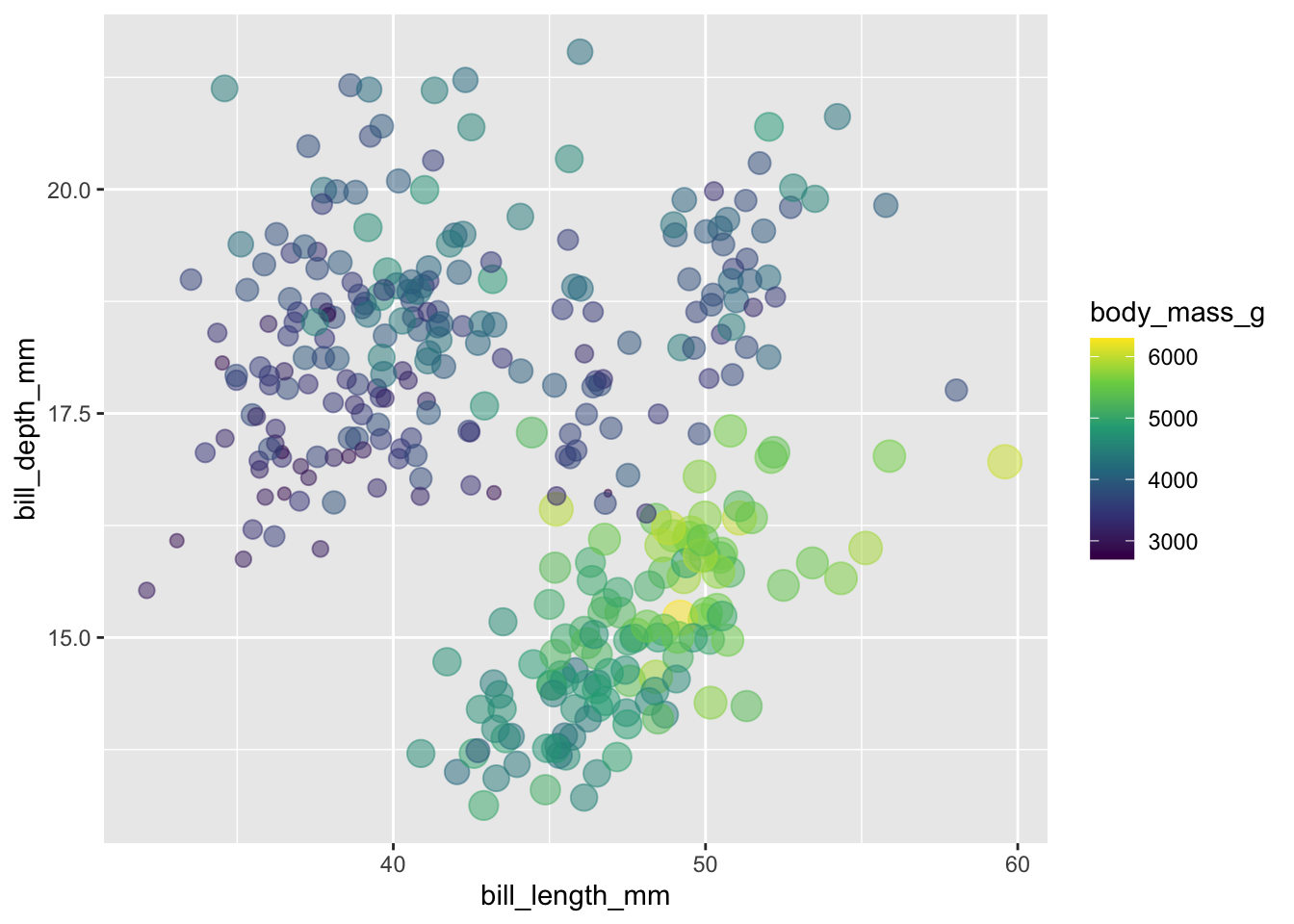
Do we think there might be an interaction between bill depth and bill length? We can try to visualise potential effects using ggplot.

Where are the heaviest penguins on the plot in relation to bill_length_mm?
And, what happens to the body weight of penguins in that range who had deeper bills (going up on the y-axis?).

Maybe there is a relationship between these two variables that we could explore in a regression model?

ggplot(drop_na(penguins), aes(y = bill_depth_mm, x = bill_length_mm, size = body_mass_g, color = body_mass_g)) + 
  geom_jitter(alpha = .5) + 
  scale_color_viridis_c() +
  scale_size_continuous(guide = 'none')

We can also explore the correlation between the two variables, here we see they are negatively correlated. This doesn’t guarantee there is an interaction, but we do see they covary!

cor.test(penguins$bill_depth_mm, penguins$bill_length_mm)

## 
##  Pearson's product-moment correlation
## 
## data:  penguins$bill_depth_mm and penguins$bill_length_mm
## t = -4.4591, df = 340, p-value = 1.12e-05
## alternative hypothesis: true correlation is not equal to 0
## 95 percent confidence interval:
##  -0.3328072 -0.1323004
## sample estimates:
##        cor 
## -0.2350529

fitting models for an interaction

Let’s z-score the variables so that we can put them on the same metric / interpretation.

# create manual z-scored versions
penguins <- drop_na(penguins) %>%
  mutate(bill_depth_z = (bill_depth_mm - mean(bill_depth_mm)) / sd(bill_depth_mm), 
         bill_length_z = (bill_length_mm - mean(bill_length_mm)) / sd(bill_length_mm))

simple effects models

Here I will fit 3 models: one per each \(X\) individually, plus a third model with both \(X\) fit as main effets:

m1 <- lm(body_mass_g ~ bill_depth_z, data = penguins)
m2 <- lm(body_mass_g ~ bill_length_z, data = penguins)
m3 <- lm(body_mass_g ~ bill_depth_z + bill_length_z, data = penguins)

Remind yourself of what this output means - bill depth has a significant relationship with penguin body weight…

summary(m1)

## 
## Call:
## lm(formula = body_mass_g ~ bill_depth_z, data = penguins)
## 
## Residuals:
##      Min       1Q   Median       3Q      Max 
## -1616.08  -510.38   -68.67   486.51  1811.12 
## 
## Coefficients:
##              Estimate Std. Error t value Pr(>|t|)    
## (Intercept)   4207.06      38.96 107.986   <2e-16 ***
## bill_depth_z  -380.07      39.02  -9.741   <2e-16 ***
## ---
## Signif. codes:  0 '***' 0.001 '**' 0.01 '*' 0.05 '.' 0.1 ' ' 1
## 
## Residual standard error: 710.9 on 331 degrees of freedom
## Multiple R-squared:  0.2228, Adjusted R-squared:  0.2205 
## F-statistic: 94.89 on 1 and 331 DF,  p-value: < 2.2e-16

As does bill length…

summary(m2)

## 
## Call:
## lm(formula = body_mass_g ~ bill_length_z, data = penguins)
## 
## Residuals:
##      Min       1Q   Median       3Q      Max 
## -1759.38  -468.82    27.79   464.20  1641.00 
## 
## Coefficients:
##               Estimate Std. Error t value Pr(>|t|)    
## (Intercept)    4207.06      35.70  117.85   <2e-16 ***
## bill_length_z   474.64      35.75   13.28   <2e-16 ***
## ---
## Signif. codes:  0 '***' 0.001 '**' 0.01 '*' 0.05 '.' 0.1 ' ' 1
## 
## Residual standard error: 651.4 on 331 degrees of freedom
## Multiple R-squared:  0.3475, Adjusted R-squared:  0.3455 
## F-statistic: 176.2 on 1 and 331 DF,  p-value: < 2.2e-16

And they both remain significant when added together, but have been adjusted based on coexisting within the model space:

Do you remember how to interpret these coefficients?

The intercept is the predicted body weight when both \(X\) are held at 0 - what does 0 mean when they are z-scored?
for each standardized increase in bill depth, body weight decreases by 287 grams
for each standardized increase in bill length, body weight increases by 409 grams

summary(m3)

## 
## Call:
## lm(formula = body_mass_g ~ bill_depth_z + bill_length_z, data = penguins)
## 
## Residuals:
##      Min       1Q   Median       3Q      Max 
## -1806.74  -456.82    15.33   471.07  1541.34 
## 
## Coefficients:
##               Estimate Std. Error t value Pr(>|t|)    
## (Intercept)    4207.06      32.30 130.257  < 2e-16 ***
## bill_depth_z   -286.54      33.23  -8.624 2.76e-16 ***
## bill_length_z   409.13      33.23  12.313  < 2e-16 ***
## ---
## Signif. codes:  0 '***' 0.001 '**' 0.01 '*' 0.05 '.' 0.1 ' ' 1
## 
## Residual standard error: 589.4 on 330 degrees of freedom
## Multiple R-squared:  0.4675, Adjusted R-squared:  0.4642 
## F-statistic: 144.8 on 2 and 330 DF,  p-value: < 2.2e-16

As a reminder, the slopes / coefficients for either \(X\) do not change when values of the other \(X\) change. This means we are not capturing the effect of \(X_1\) at different levels of \(X_2\) (or the other way around).

fitting the interaction

So how do we fit an interaction term? We simply use multiplication. The effects of \(X_1\) and \(X_2\) are literally multiplied to create a new effect. The inclusion of a multiplication term will introduce the combined and joint effects of the variables above their additive effects.

The formula for an interaction is:

\[ \large Y \sim b_0 + (b_1*X_1) + (b_2*X_2) + b_3 * (X_1 * X_2) + \epsilon \] The new coefficient term, \(b_3\), captures the joint contribution of both variables on \(Y\). This new term is used to determine how \(X_1\) or \(X_2\) will influence \(Y\) at different levels of either \(X\).

So to fit an interaction term, we type this:

m4 <- lm(body_mass_g ~ bill_depth_z*bill_length_z, data = penguins)

And inspect the model per normal:

summary(m4)

## 
## Call:
## lm(formula = body_mass_g ~ bill_depth_z * bill_length_z, data = penguins)
## 
## Residuals:
##     Min      1Q  Median      3Q     Max 
## -1814.0  -353.6     2.9   352.4  1603.6 
## 
## Coefficients:
##                            Estimate Std. Error t value Pr(>|t|)    
## (Intercept)                 4117.91      28.90 142.501  < 2e-16 ***
## bill_depth_z                -205.16      29.47  -6.961 1.84e-11 ***
## bill_length_z                522.15      30.34  17.211  < 2e-16 ***
## bill_depth_z:bill_length_z  -391.10      35.84 -10.911  < 2e-16 ***
## ---
## Signif. codes:  0 '***' 0.001 '**' 0.01 '*' 0.05 '.' 0.1 ' ' 1
## 
## Residual standard error: 505.8 on 329 degrees of freedom
## Multiple R-squared:  0.609,  Adjusted R-squared:  0.6054 
## F-statistic: 170.8 on 3 and 329 DF,  p-value: < 2.2e-16

interpreting the coefficients as conditional effects

The intercept differs because we have added a new term: the interaction between the two variables. This interaction alters how the predictors relate to the outcome depending on the value of each other variable.

As a result, the coefficients for the predictors (bill_depth and bill_length) can no longer be interpreted as main effects. Instead, they represent conditional effects, meaning their interpretation depends on the value of the other predictor.

The effect (or slope) of a +1 SD increase in bill_depth is associated with a decrease of 205 grams in body mass when bill_length is at its mean.
- (This is the conditional part: the effect is conditional on bill_length being at its mean.)
Similarly, the slope of a +1 SD increase in bill_length is associated with a 522-gram increase in body mass when bill_depth is at its mean.

interpreting the interaction term as adjustment to conditional effects

The interaction term quantifies how the relationship between each predictor and \(Y\) changes depending on the value of the other predictor.

If bill_depth increases by one unit (e.g., 1 SD in this case), the slope of bill_length decreases by 391 grams.
Similarly, if bill_length increases by one unit, the slope of bill_depth decreases by 391 grams.

This reflects the reciprocal nature of the interaction term: each predictor’s effect on \(Y\) depends on the level of the other predictor.

The interaction term modifies the slope, not the coefficient values of the main effects directly. The interaction tells us how the slope of one predictor changes as the value of the other predictor increases.

visualising the interaction

Visualising the interaction helps to demonstrate this. There are various ways to visualise interactions - a quick way is to use the plot_model function from the sjPlot library.

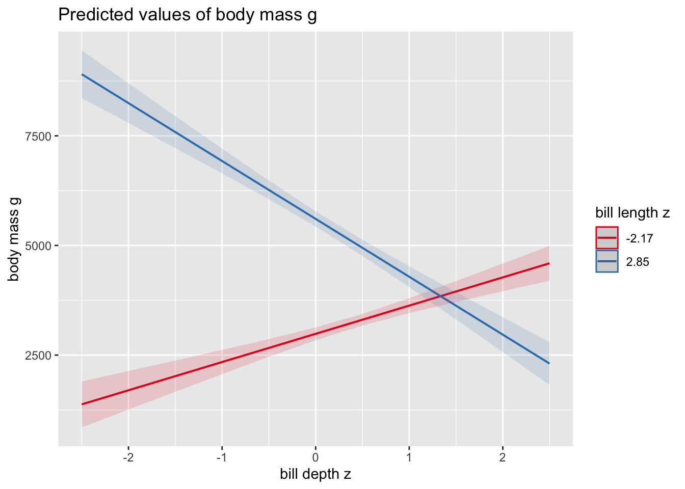
How do we interpret this plot? The two lines represent the conditional effects of bill_depth (on the x-axis) at two different levels of bill_length (the legend).

We can see that when bill_length_z = -2.17, the slope for bill_depth_z is positive
When bill_length_z = 2.85, the slope for bill_depth_z is negative

So if someone asked you whether penguin body weight is affected by bill depth, you’d say “yes, but the effect depends (or is conditional) on the length of the penguin’s bill!

library(sjPlot)

## #refugeeswelcome

# plot the interaction
plot_model(m4, type = 'int')

What are these two values of -2.18 and 2.85? They are the smallest and largest values for this variable in the raw data:

min(penguins$bill_length_z)

## [1] -2.174715

max(penguins$bill_length_z)

## [1] 2.853932

better(?) plots

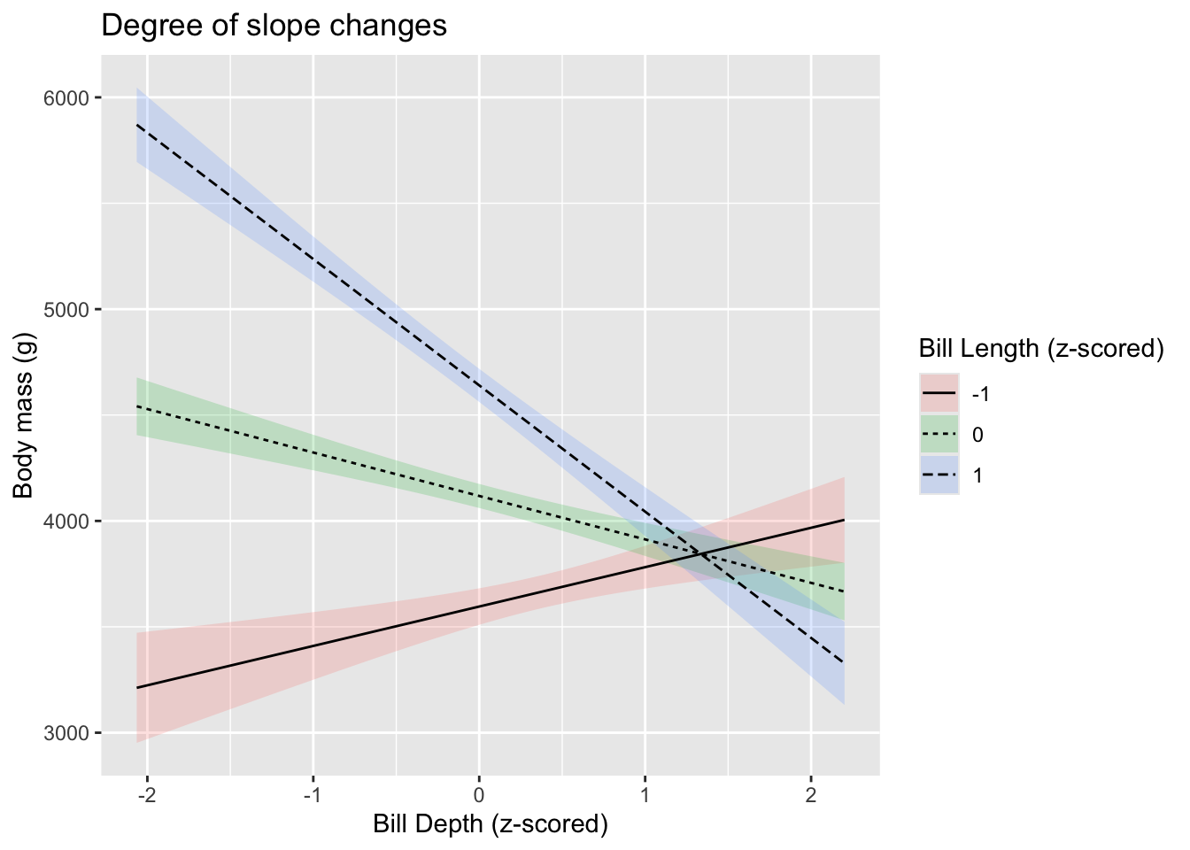
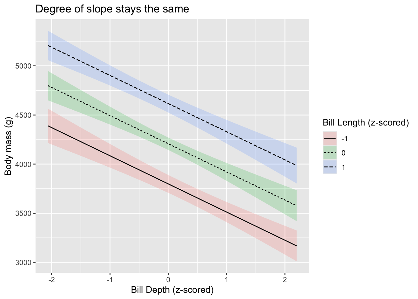
The sjPlot package picks the min/max values for us. Using more sophisticated methods from libraries such as emmeans, we can pick and choose to display the effects of one \(X\) at any level of the other variable. On choice might be to show the effect of \(X_1\) while \(X_1\) is at its mean, as well as +/- 1SD from the mean. Compare this to the earlier plot, where the slope remained the same.

what makes the interaction significant?

Whether the interaction term is “significant” is the same as any other test - whether the estimate / standard error is far enough away from zero to reach a p value below .05.

But we can also look at the model fit in terms of R2 change and other metrics:

Compare the r2 of the models with and without the interaction term:

summary(m3)$r.squared

## [1] 0.4674645

summary(m4)$r.squared

## [1] 0.6089661

There is a formal way to test the fit of two “nested” models using the anova() function

anova(m3, m4)

## Analysis of Variance Table
## 
## Model 1: body_mass_g ~ bill_depth_z + bill_length_z
## Model 2: body_mass_g ~ bill_depth_z * bill_length_z
##   Res.Df       RSS Df Sum of Sq      F    Pr(>F)    
## 1    330 114633409                                  
## 2    329  84173822  1  30459587 119.05 < 2.2e-16 ***
## ---
## Signif. codes:  0 '***' 0.001 '**' 0.01 '*' 0.05 '.' 0.1 ' ' 1

predicting a new case with the formula

Let’s say we have a penguin with a bill depth of 22mm and bill length of 50mm. What would their predicted body weight be? We use the same approach, with this formula. First we’d have to z-score the values (since the model predictions are based on z-scores).

(22-mean(penguins$bill_depth_mm)) / sd(penguins$bill_depth_mm)

## [1] 2.455336

(50-mean(penguins$bill_length_mm)) / sd(penguins$bill_length_mm)

## [1] 1.098477

\[ \large Y \sim b_0 + (b_1*X_1) + (b_2*X_2) + b_3 * (X_1 * X_2) \]

summary(m4)

## 
## Call:
## lm(formula = body_mass_g ~ bill_depth_z * bill_length_z, data = penguins)
## 
## Residuals:
##     Min      1Q  Median      3Q     Max 
## -1814.0  -353.6     2.9   352.4  1603.6 
## 
## Coefficients:
##                            Estimate Std. Error t value Pr(>|t|)    
## (Intercept)                 4117.91      28.90 142.501  < 2e-16 ***
## bill_depth_z                -205.16      29.47  -6.961 1.84e-11 ***
## bill_length_z                522.15      30.34  17.211  < 2e-16 ***
## bill_depth_z:bill_length_z  -391.10      35.84 -10.911  < 2e-16 ***
## ---
## Signif. codes:  0 '***' 0.001 '**' 0.01 '*' 0.05 '.' 0.1 ' ' 1
## 
## Residual standard error: 505.8 on 329 degrees of freedom
## Multiple R-squared:  0.609,  Adjusted R-squared:  0.6054 
## F-statistic: 170.8 on 3 and 329 DF,  p-value: < 2.2e-16

First put the intercept and coefficients into the formula:

\[ \large \text{body weight} = 4117.91 + (-205.16*X_1) + (522.15*X_2) + -391 * (X_1 * X_2) \]

Now put our new values in (remember, we z-scored them)

\[ \large \text{body weight} = 4117.91 + (-205.16* 2.455) + (522.15*1.099) + -391 * (2.455 * 1.099) \]

Then complete the calculation:

\[ \large \text{body weight} = 4117.91 + (-503.6678) + (573.8428) + (-391 * (2.698)) \] Another step…

\[ \large \text{body weight} = 4117.91 + (-503.6678) + (573.8428) + -1054.918 \]

The final step…

\[ \large \text{body weight} = 3133.167 \]

continuous by continuous interaction

2024-12-19