correlations
2025-08-14
Correlation is a measure of covariance
A correlation is a common way to measure the strength of a relationship between two continuous variables. More precisely, a correlation measures the degree to which two continuous variables co-vary (called their covariance). Put differently, a correlation determines how much two variables will change together.
Correlation values range from -1 to 1
The canonical correlation is the Pearson correlation coefficient, normally represented by \(r\). Values for \(r\) will range from -1 to 1. Negative values mean variables co-vary in different directions: as one goes up, the other goes down. Positive values means that they go in the same direction: as one goes up or down, the other goes up or down.
Let’s look at the Pearson correlation between penguin body mass and penguin flipper length:
Method 1: using cor
The cor function asks for two numeric vectors and
returns the \(r\)
The use = 'complete.obs' tells the function to ignore NA
values.
## [1] 0.8712018Method 2: using cor.test
The cor.test function provides us with more information
right away. We receive a test statistic (t) the degrees of freedom (df),
a p-value, 95% confidence interval, and the \(r\)
##
##  Pearson's product-moment correlation
##
## data:  penguins$body_mass_g and penguins$flipper_length_mm
## t = 32.722, df = 340, p-value < 2.2e-16
## alternative hypothesis: true correlation is not equal to 0
## 95 percent confidence interval:
##  0.843041 0.894599
## sample estimates:
##       cor
## 0.8712018
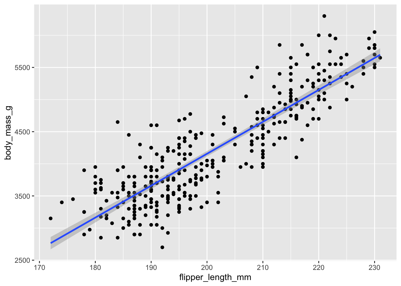
A positive correlation of 0.87 is strong (the maximum being 1.0). It indicates there is a strong positive relationship between the two variables. Plotting the regression line shows this relationship - if the line was perfectly diagonal, then \(r\) would be 1.0.
ggplot(penguins, aes(y = body_mass_g, x = flipper_length_mm)) +
  geom_point() +
  geom_smooth(method = 'lm')
## `geom_smooth()` using formula = 'y ~ x'
How do we obtain \(r\) ?
To calculate the covariance of two continuous variables, we need to put the variables on the same scale and then observe differences between the values. We already know how to put variables on the same scale using z-scores.
A Pearson correlation will:
- z-score the variables
- multiply the z-scores
- sum the products of the z-scores
- calculate an adjusted mean of the products (divide this sum by n-1)
The adjusted mean is the correlation coefficient.
Let’s look at a toy example first using short vectors:
## [1] 10 20 30 4 5 6## [1] 4 5 6 10 20 30Manually z-score the vectors:
## [1] -0.2406741 0.7220222 1.6847184 -0.8182918 -0.7220222 -0.6257526## [1] -0.8182918 -0.7220222 -0.6257526 -0.2406741 0.7220222 1.6847184We then obtain their products, which R lets us do quite easily:
## [1] 0.1969416 -0.5213160 -1.0542169 0.1969416 -0.5213160 -1.0542169Now that we have obtained products of the z-scored data, we can calculate the average of these products using an adjusted n-size:
What is the correlation?
## [1] -0.5514365Let’s check our work:
##
##  Pearson's product-moment correlation
##
## data:  v1 and v2
## t = -1.322, df = 4, p-value = 0.2567
## alternative hypothesis: true correlation is not equal to 0
## 95 percent confidence interval:
##  -0.9416060  0.4708349
## sample estimates:
##        cor
## -0.5514365
a one predictor lm is a correlation when you z-score \(y\) and \(x\)
Understanding what the correlation is doing gives us a better understanding of what a regression is doing. Indeed, a linear regression with a scaled dv and predictor will produce the correlation coefficient as the model estimate. Let’s try it out with penguin body mass and flipper length:
First, z-score the variables:
penguins$body_mass_g_z <- (penguins$body_mass_g -
                             mean(penguins$body_mass_g, na.rm = T)) /
  sd(penguins$body_mass_g, na.rm = T)

penguins$flipper_length_mm_z <- (penguins$flipper_length_mm -
                                   mean(penguins$flipper_length_mm, na.rm = T)) /
  sd(penguins$flipper_length_mm, na.rm = T)
Then fit a linear model:
The estimate is 0.871 - the exact same as the correlation coefficient
##
## Call:
## lm(formula = body_mass_g_z ~ flipper_length_mm_z, data = penguins)
##
## Residuals:
##      Min       1Q   Median       3Q      Max
## -1.32027 -0.32330 -0.03352  0.30841  1.60693
##
## Coefficients:
##                      Estimate Std. Error t value Pr(>|t|)
## (Intercept)         1.025e-15  2.659e-02    0.00        1
## flipper_length_mm_z 8.712e-01  2.662e-02   32.72   <2e-16 ***
## ---
## Signif. codes:  0 '***' 0.001 '**' 0.01 '*' 0.05 '.' 0.1 ' ' 1
##
## Residual standard error: 0.4916 on 340 degrees of freedom
##   (2 observations deleted due to missingness)
## Multiple R-squared:  0.759,  Adjusted R-squared:  0.7583
## F-statistic:  1071 on 1 and 340 DF,  p-value: < 2.2e-16
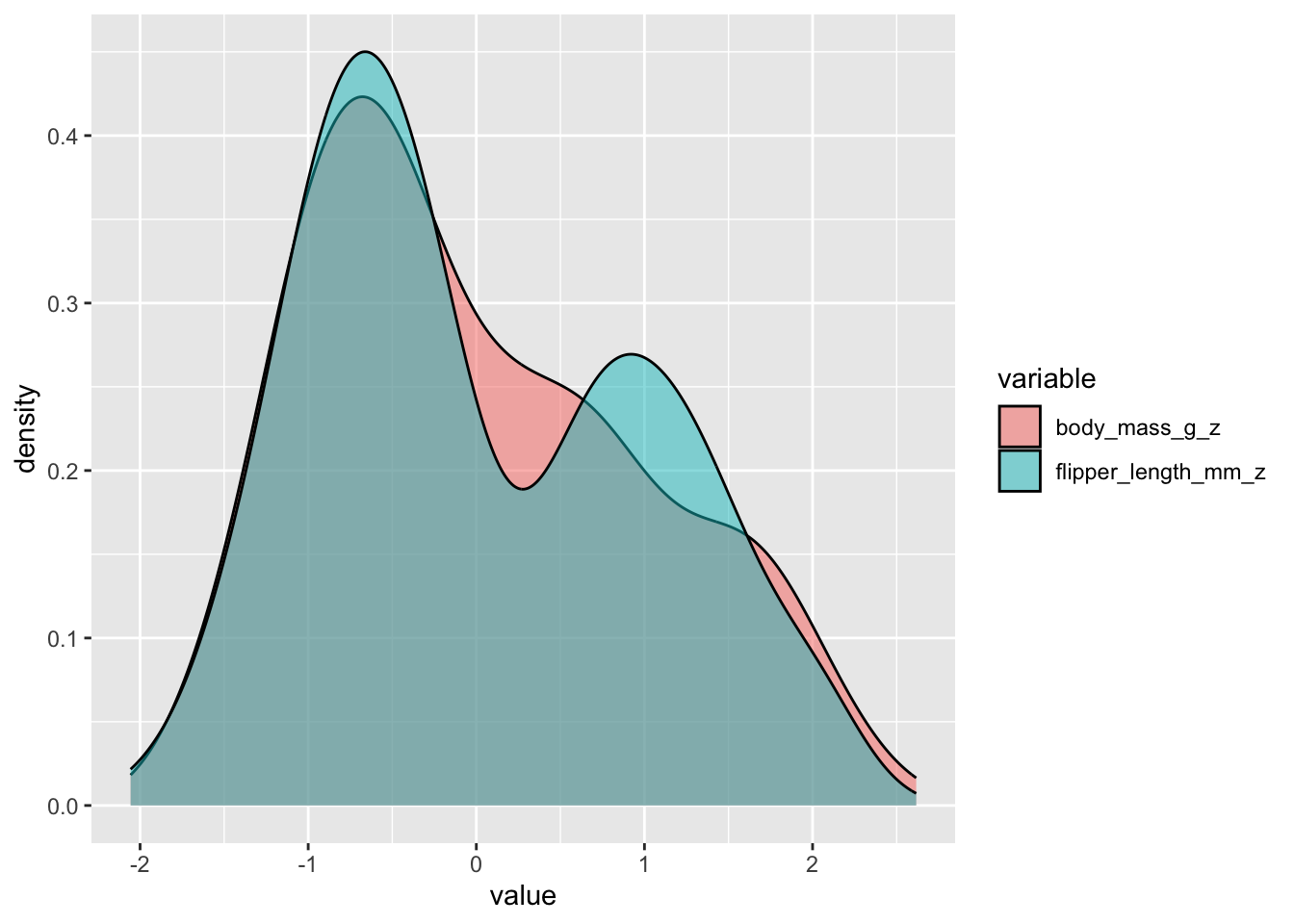
visualise this covariance:
Let’s plot the two distributios over one another to visualise the covariance:

Conclusion
There you have it - a correlation is a measure of covariance between two variables once they are standardized.
A linear regression will apply the same logic to see how predictors influence an outcome variable. When you add more than one predictor to a regression, the model will obtain the covariance of more than one variable, quickly increasing the complexity of the calculations.