Counting and describing data

This notebook introduces two new functions: group_by() and summarise(). The first function, group_by(), is used to first tell a tibble/dataframe your set of grouping variables, i.e., what do you want to group by. The second function, summarise(), will allow you to ask for any number of functions applied to your data based on that grouping structure. To demonstrate, let’s look at some penguins!

Load tidyverse and the palmerpenguins data set

library(tidyverse)
library(palmerpenguins)
data(penguins)

obtaining mean values for different species of `penguins`

We can calculate the average/mean of a variable using the base function mean(). This function takes a vector of numbers or a dataframe column and returns the average/mean. Lets use it to find the average body mass of the penguins.

# calculate the mean body mass, but what happens?
mean(penguins$body_mass_g)

## [1] NA

There is at least one NA value in the dataframe, so the function is returning NA. We can deal with this by using the na.rm argument in mean. The default value of na.rm is FALSE, meaning that NA values will not be removed. Set the argument to TRUE in order to remove the NA values from the calculations

mean(penguins$body_mass_g, na.rm = TRUE)

## [1] 4201.754

After removing the NA values, we see that the average body mass of the penguins is about 4200 grams. However, in the notebook using filter(), we developed a hypothesis that certain species of penguins had higher body masses than others. Let’s confirm this hypothesis by using mean() on three filtered versions of the data.

# here are the different species
summary(penguins$species)

##    Adelie Chinstrap    Gentoo 
##       152        68       124

In the line below, I wrap mean() around a filter() call to penguins, which asks for just the "Adelie" penguins. I also attach the $ to the end of the filter function to call just the body_mass_g column. I include na.rm = TRUE to filter out NA.

So this line of code is saying “Give me the mean of the column body_mass_g in the penguins data after filtering all rows where species is equal to ‘Adelie’ and also remove NA values during the calculation of the mean”. While this is “efficient” in being a single line, it can be a bit difficult to take in if you are unfamiliar with the different parts of the R syntax. (This is a pedagogical decision, we will see later how group_by() and summarise() improve on this.)

mean(filter(penguins, species == 'Adelie')$body_mass_g, na.rm = TRUE)

## [1] 3700.662

We see that the average body mass of the Adelie penguins is lower than the average body mass of all the penguins. Let’s quickly look at the average body mass of the other two species:

mean(filter(penguins, species == 'Chinstrap')$body_mass_g, na.rm = TRUE)

## [1] 3733.088

mean(filter(penguins, species == 'Gentoo')$body_mass_g, na.rm = TRUE)

## [1] 5076.016

It seems both the Adelie and Chinstrap penguins have a lower average body mass than the entire population average, whereas the Gentoo penguins are heavier. To understand this, we repeated the same thing three times, which is usually a signal that we could be more efficient. Moreover, we only see the means one-at-a-time. It would be far more useful to obtain all of this information at the same time. This is where group_by() and summarise() come in handy!

let’s group stuff!

The first thing we need to think about is what our grouping variable will be. In this case, it should be relatively obvious that it is species (this is the variable we used filter() on three times). Knowing this, we can start to build group_by() pipe.

It’s usually good to create a new tibble that contains your summary data. Let’s create a new variable called bm_summary, which is a copy of penguins. Then pipe into the group_by() function. We want to group by species, so add that into the group_by() function.

Let’s start with the penguins data and pipe into group_by(), like this:

bm_summary <- penguins %>%
  group_by(species)

Running this code doesn’t seem to do anything, but we have now create a new tibble which contains metadata about a grouping structure imposed on the data. You can verify this using glimpse(), which now contains a Groups output.

glimpse(bm_summary)

## Rows: 344
## Columns: 8
## Groups: species [3]
## $ species           <fct> Adelie, Adelie, Adelie, Adelie, Adelie, Adelie, Adel…
## $ island            <fct> Torgersen, Torgersen, Torgersen, Torgersen, Torgerse…
## $ bill_length_mm    <dbl> 39.1, 39.5, 40.3, NA, 36.7, 39.3, 38.9, 39.2, 34.1, …
## $ bill_depth_mm     <dbl> 18.7, 17.4, 18.0, NA, 19.3, 20.6, 17.8, 19.6, 18.1, …
## $ flipper_length_mm <int> 181, 186, 195, NA, 193, 190, 181, 195, 193, 190, 186…
## $ body_mass_g       <int> 3750, 3800, 3250, NA, 3450, 3650, 3625, 4675, 3475, …
## $ sex               <fct> male, female, female, NA, female, male, female, male…
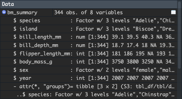
## $ year              <int> 2007, 2007, 2007, 2007, 2007, 2007, 2007, 2007, 2007…

You can also look at the tibble in the environment pane to see the grouping structure:

You can use the ungroup() function to remove this grouping structure.

# The Group information is gone now. 
bm_summary <- penguins %>%
  group_by(species) %>%
  ungroup() %>%
  glimpse()

## Rows: 344
## Columns: 8
## $ species           <fct> Adelie, Adelie, Adelie, Adelie, Adelie, Adelie, Adel…
## $ island            <fct> Torgersen, Torgersen, Torgersen, Torgersen, Torgerse…
## $ bill_length_mm    <dbl> 39.1, 39.5, 40.3, NA, 36.7, 39.3, 38.9, 39.2, 34.1, …
## $ bill_depth_mm     <dbl> 18.7, 17.4, 18.0, NA, 19.3, 20.6, 17.8, 19.6, 18.1, …
## $ flipper_length_mm <int> 181, 186, 195, NA, 193, 190, 181, 195, 193, 190, 186…
## $ body_mass_g       <int> 3750, 3800, 3250, NA, 3450, 3650, 3625, 4675, 3475, …
## $ sex               <fct> male, female, female, NA, female, male, female, male…
## $ year              <int> 2007, 2007, 2007, 2007, 2007, 2007, 2007, 2007, 2007…

let’s summarise stuff!

Okay, now that we can group, let’s use summarise() to obtain the mean of each level of our grouping variable. To do so, pipe into a summarise() function after the group_by() function.

The summarise() function works similar to mutate(). We create new values, so we first give our value a new name. Call the new value mean_body_mass. We then set the value to be the result of calling some sort of function on a column. In this case, we want to call mean() on body_mass_g. Don’t forget to include na.rm = TRUE !

bm_summary <- penguins %>%
  group_by(species) %>%
  summarise(mean_body_mass = mean(body_mass_g, na.rm = TRUE)) %>%
  glimpse()

## Rows: 3
## Columns: 2
## $ species        <fct> Adelie, Chinstrap, Gentoo
## $ mean_body_mass <dbl> 3700.662, 3733.088, 5076.016

Notice what happens to the tibble, it’s now 3 rows long and 2 columns wide. If you look at the data in the data viewer, you see something like this:

So the two remaining columns are (1) the column which was included in group_by() and (2) the new variable that was created. We have reduced (or summarised) our tibble into a smaller set of data. And, moreover, we can clearly see the 3 means for the 3 species in one place. Calling the name of the tibble prints this information straight to the console for us, neat!

bm_summary

## # A tibble: 3 × 2
##   species   mean_body_mass
##   <fct>              <dbl>
## 1 Adelie             3701.
## 2 Chinstrap          3733.
## 3 Gentoo             5076.

creating multiple values in `summarise()`

Just like mutate(), we can create as many variables as we want within a single summarise() function. Let’s try that now. When we report the mean/average of something, we usually also report the standard deviation. You can obtain the standard deviation in R using the sd() function. With this knowledge, let’s create a new variable called sd_body_mass alongside the mean. It will also require the na.rm = TRUE command

bm_summary <- penguins %>%
  group_by(species) %>%
  summarise(mean_body_mass = mean(body_mass_g, na.rm = TRUE), 
            sd_body_mass = sd(body_mass_g, na.rm = TRUE)) %>%
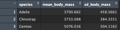
  glimpse()

## Rows: 3
## Columns: 3
## $ species        <fct> Adelie, Chinstrap, Gentoo
## $ mean_body_mass <dbl> 3700.662, 3733.088, 5076.016
## $ sd_body_mass   <dbl> 458.5661, 384.3351, 504.1162

Just as before, there are 3 rows (one per level of species), but now we also have 3 columns. This should make sense, since we asked for a third value (standard deviation). Your data should look something like this:

Keep going! Add the min() and max() values to the data, all inside the same summarise() call. Give the new variables the names min_body_mass and max_body_mass:

bm_summary <- penguins %>%
  group_by(species) %>%
  summarise(mean_body_mass = mean(body_mass_g, na.rm = TRUE), 
            sd_body_mass = sd(body_mass_g, na.rm = TRUE),
            min_body_mass = min(body_mass_g, na.rm = TRUE),
            max_body_mass = max(body_mass_g, na.rm = TRUE)) %>%
  glimpse()

## Rows: 3
## Columns: 5
## $ species        <fct> Adelie, Chinstrap, Gentoo
## $ mean_body_mass <dbl> 3700.662, 3733.088, 5076.016
## $ sd_body_mass   <dbl> 458.5661, 384.3351, 504.1162
## $ min_body_mass  <int> 2850, 2700, 3950
## $ max_body_mass  <int> 4775, 4800, 6300

Just like mutate, we can operate on variables we create inside the summarise() function! So, after creating the min/max body mass columns, we could then perform a calculation to obtain the range() of the body mass (i.e., the distance between the minimum and maximum values). Instead of using a function, let’s just subtract the max from the min.

bm_summary <- penguins %>%
  group_by(species) %>%
  summarise(mean_body_mass = mean(body_mass_g, na.rm = TRUE), 
            sd_body_mass = sd(body_mass_g, na.rm = TRUE),
            min_body_mass = min(body_mass_g, na.rm = TRUE),
            max_body_mass = max(body_mass_g, na.rm = TRUE), 
            range_body_mass = max_body_mass - min_body_mass) %>%
  glimpse()

## Rows: 3
## Columns: 6
## $ species         <fct> Adelie, Chinstrap, Gentoo
## $ mean_body_mass  <dbl> 3700.662, 3733.088, 5076.016
## $ sd_body_mass    <dbl> 458.5661, 384.3351, 504.1162
## $ min_body_mass   <int> 2850, 2700, 3950
## $ max_body_mass   <int> 4775, 4800, 6300
## $ range_body_mass <int> 1925, 2100, 2350

but how do you count things?

Pretty cool right - we can create as many values as we need in order to describe our population. However, we are missing a pretty important one…counting the members of our population! A shorthand you might see for this in manuscripts and elsewhere is something like n = x. There is happily a function called n() which gives this exact information. Let’s try it out by asking for the n of our penguins species. It’s as simple as adding n = n(). I’m choosing to call it n, but we could call it anything (right?)

bm_summary <- penguins %>%
  group_by(species) %>%
  summarise(n = n(), 
            mean_body_mass = mean(body_mass_g, na.rm = TRUE), 
            sd_body_mass = sd(body_mass_g, na.rm = TRUE),
            min_body_mass = min(body_mass_g, na.rm = TRUE),
            max_body_mass = max(body_mass_g, na.rm = TRUE), 
            range_body_mass = max_body_mass - min_body_mass) %>%
  glimpse()

## Rows: 3
## Columns: 7
## $ species         <fct> Adelie, Chinstrap, Gentoo
## $ n               <int> 152, 68, 124
## $ mean_body_mass  <dbl> 3700.662, 3733.088, 5076.016
## $ sd_body_mass    <dbl> 458.5661, 384.3351, 504.1162
## $ min_body_mass   <int> 2850, 2700, 3950
## $ max_body_mass   <int> 4775, 4800, 6300
## $ range_body_mass <int> 1925, 2100, 2350

adding another grouping variable

The beauty of group_by() is that you can add any number of grouping variables to make calculations with. So, right now the summarise function has been operating across the three different types of species in the data. but what if we wanted to also know this information separated by year? It’s as simple as adding year to the group_by call. Let’s try it out and look at the population and mean body mass of penguins, by species, by year:

bm_year_summary <- penguins %>%
  group_by(species, year) %>%
  summarise(n = n(), mean_body_mass = mean(body_mass_g, na.rm = TRUE))

## `summarise()` has grouped output by 'species'.
## You can override using the `.groups` argument.

bm_year_summary

## # A tibble: 9 × 4
## # Groups:   species [3]
##   species    year     n mean_body_mass
##   <fct>     <int> <int>          <dbl>
## 1 Adelie     2007    50          3696.
## 2 Adelie     2008    50          3742 
## 3 Adelie     2009    52          3665.
## 4 Chinstrap  2007    26          3694.
## 5 Chinstrap  2008    18          3800 
## 6 Chinstrap  2009    24          3725 
## 7 Gentoo     2007    34          5071.
## 8 Gentoo     2008    46          5020.
## 9 Gentoo     2009    44          5141.

adding a third grouping variable

Repeat the above, but also include the sex variable in the summary. This has introduced a few rows where sex is NA. What is going on? (Hint, look at the full data frame and find all the NA values.)

bm_year_sex_summary <- penguins %>%
  group_by(species, year, sex) %>%
  summarise(n = n(), mean_body_mass = mean(body_mass_g, na.rm = TRUE))

## `summarise()` has grouped output by 'species',
## 'year'. You can override using the `.groups`
## argument.

bm_year_sex_summary

## # A tibble: 22 × 5
## # Groups:   species, year [9]
##    species    year sex        n mean_body_mass
##    <fct>     <int> <fct>  <int>          <dbl>
##  1 Adelie     2007 female    22          3390.
##  2 Adelie     2007 male      22          4039.
##  3 Adelie     2007 <NA>       6          3540 
##  4 Adelie     2008 female    25          3386 
##  5 Adelie     2008 male      25          4098 
##  6 Adelie     2009 female    26          3335.
##  7 Adelie     2009 male      26          3995.
##  8 Chinstrap  2007 female    13          3569.
##  9 Chinstrap  2007 male      13          3819.
## 10 Chinstrap  2008 female     9          3472.
## # ℹ 12 more rows

How do i get this information outside of R?

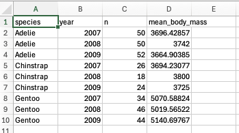
You probably want to report this summary information in a manuscript, likely even as a table. You could copy and paste this information from R into somewhere else, but why do that when you could easily output the information as a .csv file? We can do so with the write_csv() function. The function takes two main arguments - the name of the tibble you want to output, and the name you would like to give the file. So, running the cell below will output the object bm_year_summary and give it the name 'my_awesome_penguins_summary.csv'

If you don’t tell R where to save the file, it will be saved to whatever the current working directory is. If you are using an R markdown or notebook file, it should be the same directory of wherever that file is saved. You can check the current working directory using the getwd() function.

write_csv(bm_year_summary, 'my_awesome_penguins_summary.csv')

And if we were to open this up in a spreadsheet program, it might look like this:

Grouping and summarising data

2024-12-19

Counting and describing data

obtaining mean values for different species of `penguins`

let’s group stuff!

let’s summarise stuff!

creating multiple values in `summarise()`

but how do you count things?

adding another grouping variable

adding a third grouping variable

How do i get this information outside of R?

Grouping and summarising data

2024-12-19

Counting and describing data

obtaining mean values for different species of penguins

let’s group stuff!

let’s summarise stuff!

creating multiple values in summarise()

but how do you count things?

adding another grouping variable

adding a third grouping variable

How do i get this information outside of R?

obtaining mean values for different species of `penguins`

creating multiple values in `summarise()`