boxplots
2025-05-28
This notebook explains how to visualize data in R using boxplots. It
first describes how to understand a boxplot, how to create a boxplot
using base R, and then how to use the ggplot package to
create boxplots.
Load in tidyverse and the penguins data.
understanding boxplots
Visualising data is an important step for any analysis. One of the
most useful plots for continuous data is the boxplot. Base R has a
default way to create a boxplot with the boxplot()
function.
Use the boxplot function to create a boxplot of the
body_mass_g column in the penguins data:
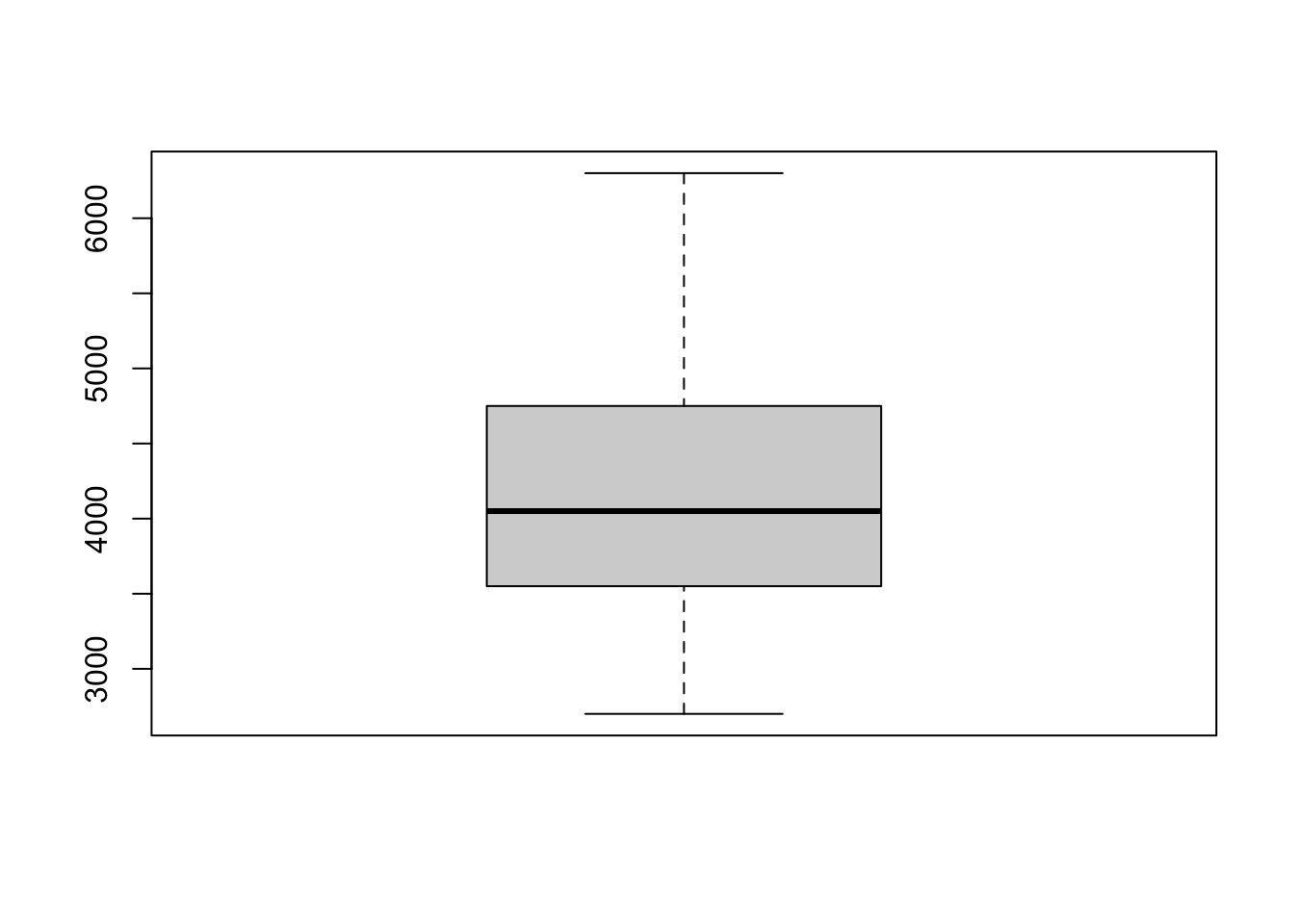
How to read a boxplot?
- the solid black line is the median. This represents
a point between 50% of the data (i.e., 50% of the data is above and 50%
of the data is below) We can obtain the median using the
median()function:
## [1] 4050what does the box mean?
The box that is in the middle of the boxplot contains the median and 50% of the total data. Specifically, it includes the first 25% of the data below and above the median. Technically, we are seeing information about the interquartile range. The bottom of the box shows where the first quarter of the data extends to (Q1), the median is the second quarter (Q2), and the top of the box is the third quarter (Q3).
what do the whiskers mean?
The whiskers are not the full range of the data. They extend
either direction from the top/bottom at a rate of 1.5 * the
interquartile range. The interquartile range is the difference between
Q3 and Q1. We can obtain Q3 and Q1 using summary()
##    Min. 1st Qu.  Median    Mean 3rd Qu.    Max.    NA's
##    2700    3550    4050    4202    4750    6300       2
So the interquartile range is 4750-3550
## [1] 1200We could also use the IQR() function to calculate the
interquartile range
## [1] 1200finding “outliers” in boxplots
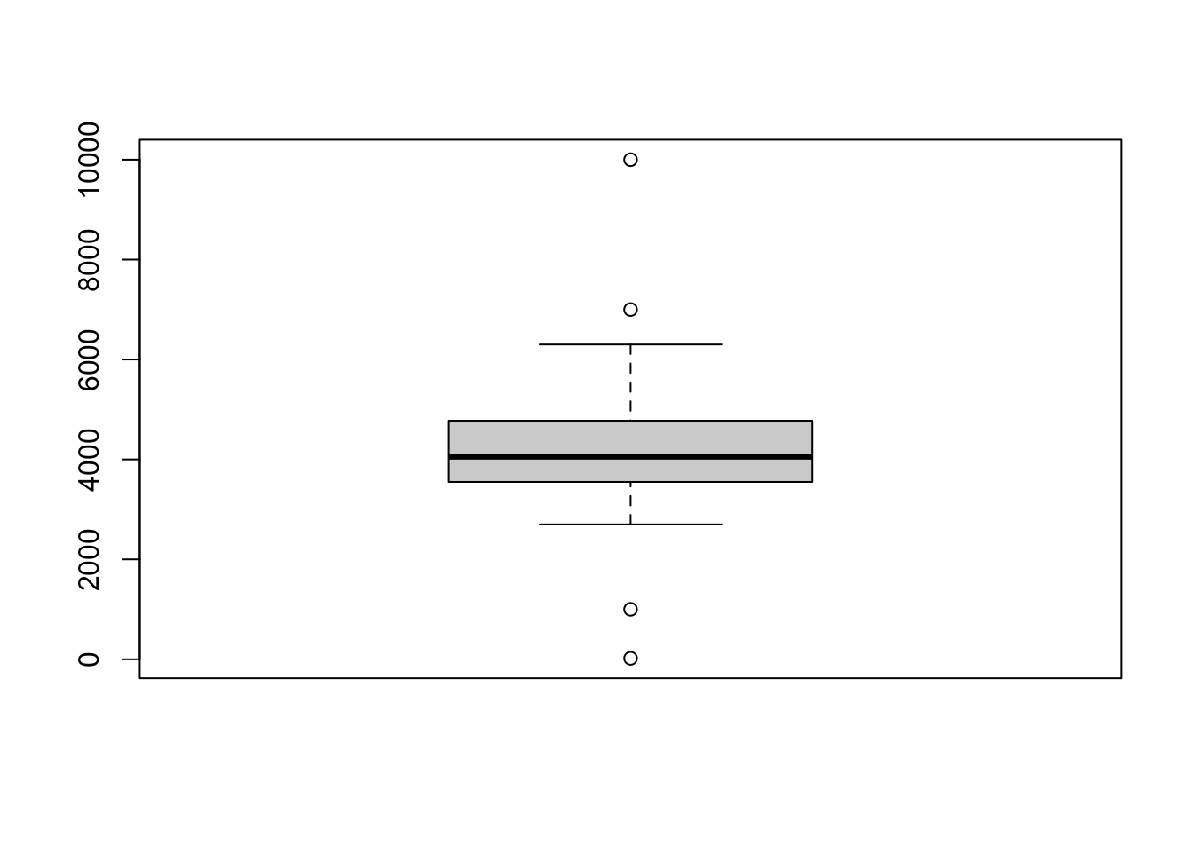
In the current boxplot, all of the data falls within the whiskers. Let’s add a few extreme points to demonstrate what happens when some points are outside the range.
The code cell below adds new values for the column
body_mass_g at row positions 345, 346, 347, and 348. The
square brackets [] index where we want to place the new
value, and take two arguments [row, column]. By only
inputting the first value, I’m telling R which row to choose, but also
saying “all columns.” Choosing the body_mass_g column with
$body_mass_g then lets me choose that specific column for
the specific row indicated in the square brackets.
# adding new rows with extreme values for body_mass_g
penguins[345,]$body_mass_g <- 1000
penguins[346,]$body_mass_g <- 20
penguins[347,]$body_mass_g <- 10000
penguins[348,]$body_mass_g <- 7000
All four values that were added are outside 1.5 * the interquartile range, and they show up as dots on the plot (sometimes called “outliers”).
So the boxplot does not always show the full range of data! And, crucially, you should know that these extreme values are part of the data distribution.
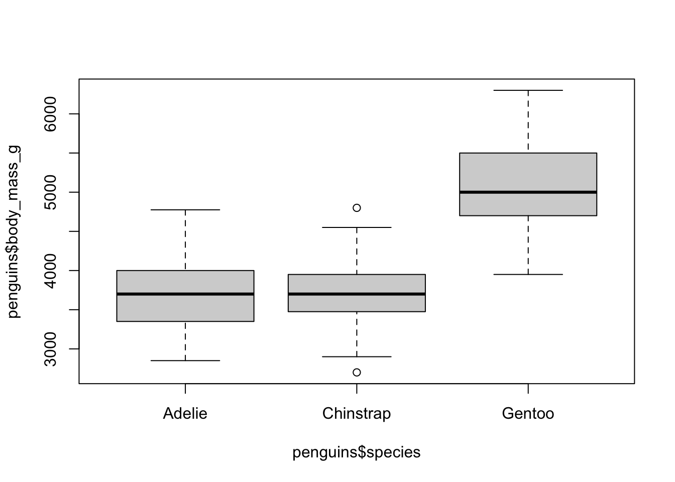
create a grouped boxplot
Let’s plot the data by species. We can do this using the formula
notation, which uses the ~ to basically stand for “by”. So
if we want to group the boxplots by species, we add a
~ and the grouping variable to the boxplot()
function:
What happens if we input the arguments the other way?
Oh my…this happens because the default argument for
boxplot() is the form of y ~ group (you can
verify this using help()). So we are telling the boxplot to
use body mass as a grouping variable, which means it will use each
unique body mass value as a group. Not ideal.
Let’s go back to the original boxplot and add some more stuff.
We can use the xlab and ylab arguments to
change the labels to something nicer than the columns of the data
frame.
# add labels for the x and y axes
boxplot(penguins$body_mass_g ~ penguins$species,
        xlab = 'Species',
        ylab = 'Body Mass (g)')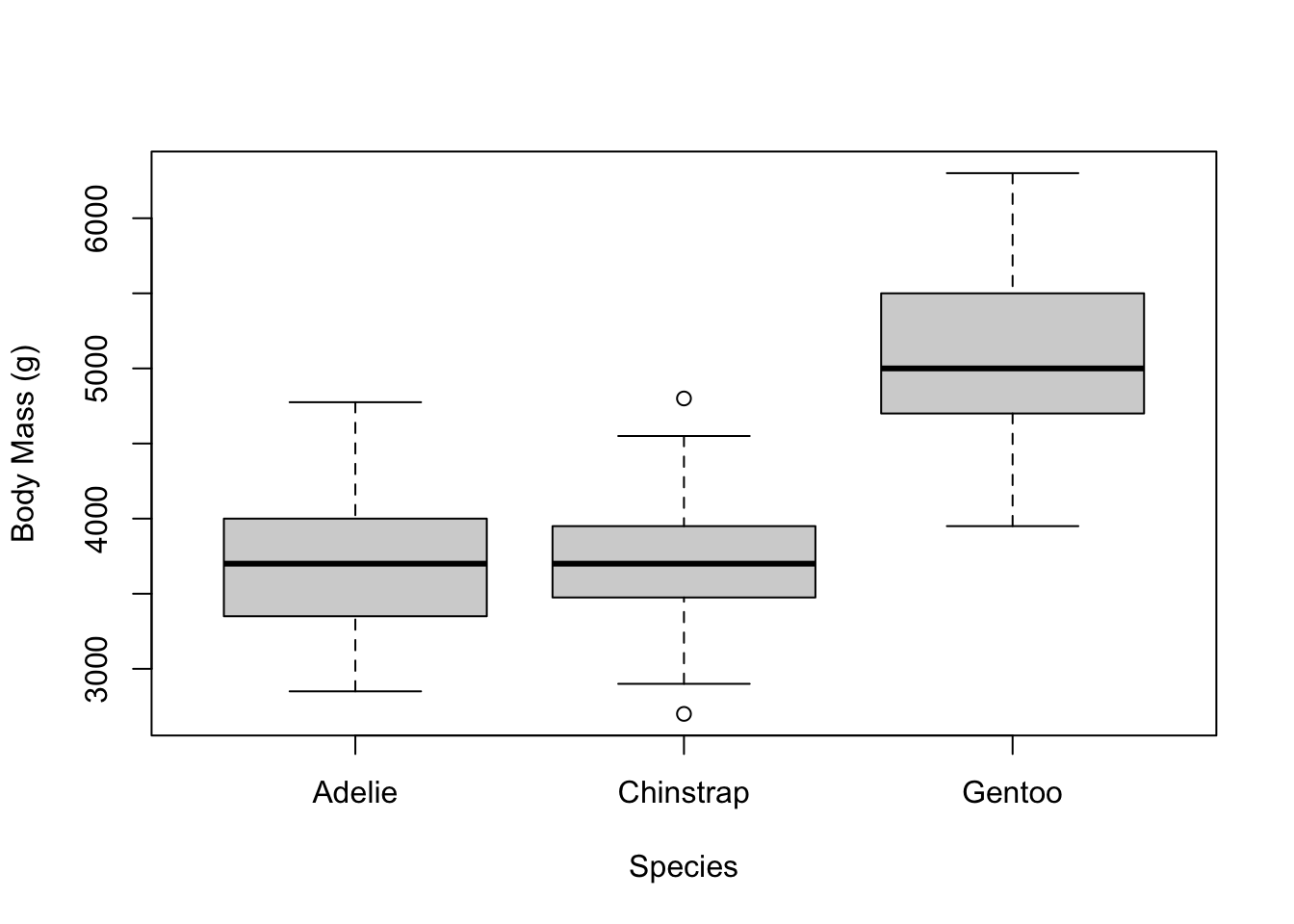
We can also turn the boxplots sideways by setting the
horizontal argument to TRUE
# turn the boxplots horizontal

boxplot(penguins$body_mass_g ~ penguins$species,
        xlab = 'Species',
        ylab = 'Body Mass (g)',
        horizontal = T)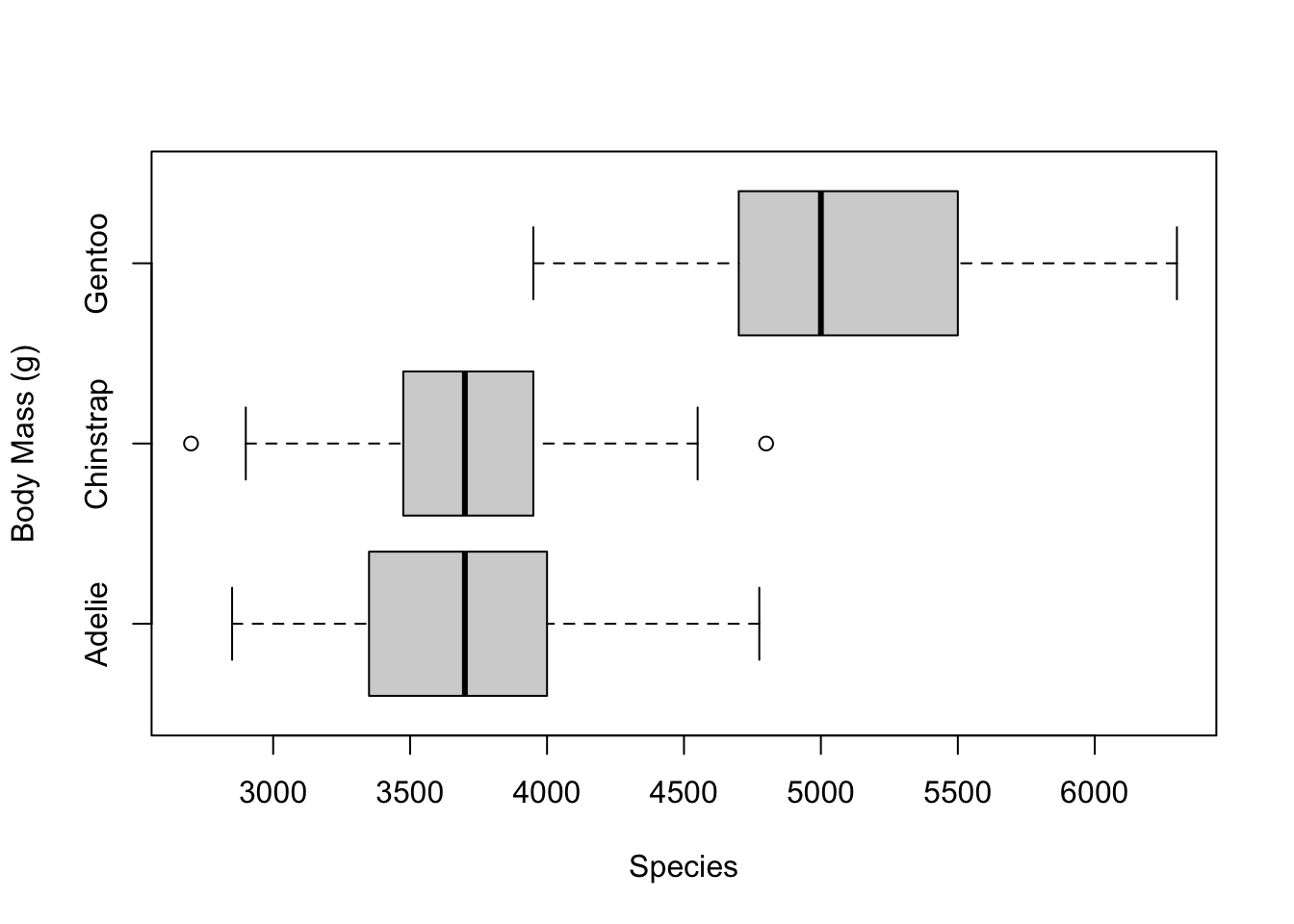
adding color
We can also add some colour to our the boxes using the
col argument. However, we need to feed col
what is known as a vector, which you can think of as a list
of values. To do that, we use the c() function, which
stands for “combine”.
creating a vector with c()
To create a vector of values, wrap them within c() and
separate them by commas. For example:
c(1,2,3)c('one', 'two', 'three')So if we want to add colors for each boxplot, we need to create a
vector of three colors and then feed that vector to the col
argument in the call to the boxplot.
boxplot(penguins$body_mass_g ~ penguins$species,
        xlab = 'Species', ylab = 'Body Mass (g)',

        col = c('lightblue','pink','forestgreen'))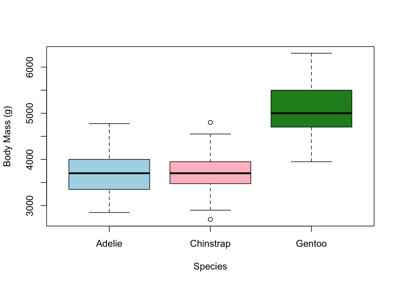
You can see all of the colors available in base R using the function
colors(). And with R Studio, you can type the name of the
color in quotes and it will show you the actual color!
## [1] "white" "aliceblue" "antiquewhite"
## [4] "antiquewhite1" "antiquewhite2" "antiquewhite3"
## [7] "antiquewhite4" "aquamarine" "aquamarine1"
## [10] "aquamarine2" "aquamarine3" "aquamarine4"
## [13] "azure" "azure1" "azure2"
## [16] "azure3" "azure4" "beige"
## [19] "bisque" "bisque1" "bisque2"
## [22] "bisque3" "bisque4" "black"
## [25] "blanchedalmond" "blue" "blue1"
## [28] "blue2" "blue3" "blue4"
## [31] "blueviolet" "brown" "brown1"
## [34] "brown2" "brown3" "brown4"
## [37] "burlywood" "burlywood1" "burlywood2"
## [40] "burlywood3" "burlywood4" "cadetblue"
## [43] "cadetblue1" "cadetblue2" "cadetblue3"
## [46] "cadetblue4" "chartreuse" "chartreuse1"
## [49] "chartreuse2" "chartreuse3" "chartreuse4"
## [52] "chocolate" "chocolate1" "chocolate2"
## [55] "chocolate3" "chocolate4" "coral"
## [58] "coral1" "coral2" "coral3"
## [61] "coral4" "cornflowerblue" "cornsilk"
## [64] "cornsilk1" "cornsilk2" "cornsilk3"
## [67] "cornsilk4" "cyan" "cyan1"
## [70] "cyan2" "cyan3" "cyan4"
## [73] "darkblue" "darkcyan" "darkgoldenrod"
## [76] "darkgoldenrod1" "darkgoldenrod2" "darkgoldenrod3"
## [79] "darkgoldenrod4" "darkgray" "darkgreen"
## [82] "darkgrey" "darkkhaki" "darkmagenta"
## [85] "darkolivegreen" "darkolivegreen1" "darkolivegreen2"
## [88] "darkolivegreen3" "darkolivegreen4" "darkorange"
## [91] "darkorange1" "darkorange2" "darkorange3"
## [94] "darkorange4" "darkorchid" "darkorchid1"
## [97] "darkorchid2" "darkorchid3" "darkorchid4"
## [100] "darkred" "darksalmon" "darkseagreen"
## [103] "darkseagreen1" "darkseagreen2" "darkseagreen3"
## [106] "darkseagreen4" "darkslateblue" "darkslategray"
## [109] "darkslategray1" "darkslategray2" "darkslategray3"
## [112] "darkslategray4" "darkslategrey" "darkturquoise"
## [115] "darkviolet" "deeppink" "deeppink1"
## [118] "deeppink2" "deeppink3" "deeppink4"
## [121] "deepskyblue" "deepskyblue1" "deepskyblue2"
## [124] "deepskyblue3" "deepskyblue4" "dimgray"
## [127] "dimgrey" "dodgerblue" "dodgerblue1"
## [130] "dodgerblue2" "dodgerblue3" "dodgerblue4"
## [133] "firebrick" "firebrick1" "firebrick2"
## [136] "firebrick3" "firebrick4" "floralwhite"
## [139] "forestgreen" "gainsboro" "ghostwhite"
## [142] "gold" "gold1" "gold2"
## [145] "gold3" "gold4" "goldenrod"
## [148] "goldenrod1" "goldenrod2" "goldenrod3"
## [151] "goldenrod4" "gray" "gray0"
## [154] "gray1" "gray2" "gray3"
## [157] "gray4" "gray5" "gray6"
## [160] "gray7" "gray8" "gray9"
## [163] "gray10" "gray11" "gray12"
## [166] "gray13" "gray14" "gray15"
## [169] "gray16" "gray17" "gray18"
## [172] "gray19" "gray20" "gray21"
## [175] "gray22" "gray23" "gray24"
## [178] "gray25" "gray26" "gray27"
## [181] "gray28" "gray29" "gray30"
## [184] "gray31" "gray32" "gray33"
## [187] "gray34" "gray35" "gray36"
## [190] "gray37" "gray38" "gray39"
## [193] "gray40" "gray41" "gray42"
## [196] "gray43" "gray44" "gray45"
## [199] "gray46" "gray47" "gray48"
## [202] "gray49" "gray50" "gray51"
## [205] "gray52" "gray53" "gray54"
## [208] "gray55" "gray56" "gray57"
## [211] "gray58" "gray59" "gray60"
## [214] "gray61" "gray62" "gray63"
## [217] "gray64" "gray65" "gray66"
## [220] "gray67" "gray68" "gray69"
## [223] "gray70" "gray71" "gray72"
## [226] "gray73" "gray74" "gray75"
## [229] "gray76" "gray77" "gray78"
## [232] "gray79" "gray80" "gray81"
## [235] "gray82" "gray83" "gray84"
## [238] "gray85" "gray86" "gray87"
## [241] "gray88" "gray89" "gray90"
## [244] "gray91" "gray92" "gray93"
## [247] "gray94" "gray95" "gray96"
## [250] "gray97" "gray98" "gray99"
## [253] "gray100" "green" "green1"
## [256] "green2" "green3" "green4"
## [259] "greenyellow" "grey" "grey0"
## [262] "grey1" "grey2" "grey3"
## [265] "grey4" "grey5" "grey6"
## [268] "grey7" "grey8" "grey9"
## [271] "grey10" "grey11" "grey12"
## [274] "grey13" "grey14" "grey15"
## [277] "grey16" "grey17" "grey18"
## [280] "grey19" "grey20" "grey21"
## [283] "grey22" "grey23" "grey24"
## [286] "grey25" "grey26" "grey27"
## [289] "grey28" "grey29" "grey30"
## [292] "grey31" "grey32" "grey33"
## [295] "grey34" "grey35" "grey36"
## [298] "grey37" "grey38" "grey39"
## [301] "grey40" "grey41" "grey42"
## [304] "grey43" "grey44" "grey45"
## [307] "grey46" "grey47" "grey48"
## [310] "grey49" "grey50" "grey51"
## [313] "grey52" "grey53" "grey54"
## [316] "grey55" "grey56" "grey57"
## [319] "grey58" "grey59" "grey60"
## [322] "grey61" "grey62" "grey63"
## [325] "grey64" "grey65" "grey66"
## [328] "grey67" "grey68" "grey69"
## [331] "grey70" "grey71" "grey72"
## [334] "grey73" "grey74" "grey75"
## [337] "grey76" "grey77" "grey78"
## [340] "grey79" "grey80" "grey81"
## [343] "grey82" "grey83" "grey84"
## [346] "grey85" "grey86" "grey87"
## [349] "grey88" "grey89" "grey90"
## [352] "grey91" "grey92" "grey93"
## [355] "grey94" "grey95" "grey96"
## [358] "grey97" "grey98" "grey99"
## [361] "grey100" "honeydew" "honeydew1"
## [364] "honeydew2" "honeydew3" "honeydew4"
## [367] "hotpink" "hotpink1" "hotpink2"
## [370] "hotpink3" "hotpink4" "indianred"
## [373] "indianred1" "indianred2" "indianred3"
## [376] "indianred4" "ivory" "ivory1"
## [379] "ivory2" "ivory3" "ivory4"
## [382] "khaki" "khaki1" "khaki2"
## [385] "khaki3" "khaki4" "lavender"
## [388] "lavenderblush" "lavenderblush1" "lavenderblush2"
## [391] "lavenderblush3" "lavenderblush4" "lawngreen"
## [394] "lemonchiffon" "lemonchiffon1" "lemonchiffon2"
## [397] "lemonchiffon3" "lemonchiffon4" "lightblue"
## [400] "lightblue1" "lightblue2" "lightblue3"
## [403] "lightblue4" "lightcoral" "lightcyan"
## [406] "lightcyan1" "lightcyan2" "lightcyan3"
## [409] "lightcyan4" "lightgoldenrod" "lightgoldenrod1"
## [412] "lightgoldenrod2" "lightgoldenrod3" "lightgoldenrod4"
## [415] "lightgoldenrodyellow" "lightgray" "lightgreen"
## [418] "lightgrey" "lightpink" "lightpink1"
## [421] "lightpink2" "lightpink3" "lightpink4"
## [424] "lightsalmon" "lightsalmon1" "lightsalmon2"
## [427] "lightsalmon3" "lightsalmon4" "lightseagreen"
## [430] "lightskyblue" "lightskyblue1" "lightskyblue2"
## [433] "lightskyblue3" "lightskyblue4" "lightslateblue"
## [436] "lightslategray" "lightslategrey" "lightsteelblue"
## [439] "lightsteelblue1" "lightsteelblue2" "lightsteelblue3"
## [442] "lightsteelblue4" "lightyellow" "lightyellow1"
## [445] "lightyellow2" "lightyellow3" "lightyellow4"
## [448] "limegreen" "linen" "magenta"
## [451] "magenta1" "magenta2" "magenta3"
## [454] "magenta4" "maroon" "maroon1"
## [457] "maroon2" "maroon3" "maroon4"
## [460] "mediumaquamarine" "mediumblue" "mediumorchid"
## [463] "mediumorchid1" "mediumorchid2" "mediumorchid3"
## [466] "mediumorchid4" "mediumpurple" "mediumpurple1"
## [469] "mediumpurple2" "mediumpurple3" "mediumpurple4"
## [472] "mediumseagreen" "mediumslateblue" "mediumspringgreen"
## [475] "mediumturquoise" "mediumvioletred" "midnightblue"
## [478] "mintcream" "mistyrose" "mistyrose1"
## [481] "mistyrose2" "mistyrose3" "mistyrose4"
## [484] "moccasin" "navajowhite" "navajowhite1"
## [487] "navajowhite2" "navajowhite3" "navajowhite4"
## [490] "navy" "navyblue" "oldlace"
## [493] "olivedrab" "olivedrab1" "olivedrab2"
## [496] "olivedrab3" "olivedrab4" "orange"
## [499] "orange1" "orange2" "orange3"
## [502] "orange4" "orangered" "orangered1"
## [505] "orangered2" "orangered3" "orangered4"
## [508] "orchid" "orchid1" "orchid2"
## [511] "orchid3" "orchid4" "palegoldenrod"
## [514] "palegreen" "palegreen1" "palegreen2"
## [517] "palegreen3" "palegreen4" "paleturquoise"
## [520] "paleturquoise1" "paleturquoise2" "paleturquoise3"
## [523] "paleturquoise4" "palevioletred" "palevioletred1"
## [526] "palevioletred2" "palevioletred3" "palevioletred4"
## [529] "papayawhip" "peachpuff" "peachpuff1"
## [532] "peachpuff2" "peachpuff3" "peachpuff4"
## [535] "peru" "pink" "pink1"
## [538] "pink2" "pink3" "pink4"
## [541] "plum" "plum1" "plum2"
## [544] "plum3" "plum4" "powderblue"
## [547] "purple" "purple1" "purple2"
## [550] "purple3" "purple4" "red"
## [553] "red1" "red2" "red3"
## [556] "red4" "rosybrown" "rosybrown1"
## [559] "rosybrown2" "rosybrown3" "rosybrown4"
## [562] "royalblue" "royalblue1" "royalblue2"
## [565] "royalblue3" "royalblue4" "saddlebrown"
## [568] "salmon" "salmon1" "salmon2"
## [571] "salmon3" "salmon4" "sandybrown"
## [574] "seagreen" "seagreen1" "seagreen2"
## [577] "seagreen3" "seagreen4" "seashell"
## [580] "seashell1" "seashell2" "seashell3"
## [583] "seashell4" "sienna" "sienna1"
## [586] "sienna2" "sienna3" "sienna4"
## [589] "skyblue" "skyblue1" "skyblue2"
## [592] "skyblue3" "skyblue4" "slateblue"
## [595] "slateblue1" "slateblue2" "slateblue3"
## [598] "slateblue4" "slategray" "slategray1"
## [601] "slategray2" "slategray3" "slategray4"
## [604] "slategrey" "snow" "snow1"
## [607] "snow2" "snow3" "snow4"
## [610] "springgreen" "springgreen1" "springgreen2"
## [613] "springgreen3" "springgreen4" "steelblue"
## [616] "steelblue1" "steelblue2" "steelblue3"
## [619] "steelblue4" "tan" "tan1"
## [622] "tan2" "tan3" "tan4"
## [625] "thistle" "thistle1" "thistle2"
## [628] "thistle3" "thistle4" "tomato"
## [631] "tomato1" "tomato2" "tomato3"
## [634] "tomato4" "turquoise" "turquoise1"
## [637] "turquoise2" "turquoise3" "turquoise4"
## [640] "violet" "violetred" "violetred1"
## [643] "violetred2" "violetred3" "violetred4"
## [646] "wheat" "wheat1" "wheat2"
## [649] "wheat3" "wheat4" "whitesmoke"
## [652] "yellow" "yellow1" "yellow2"
## [655] "yellow3" "yellow4" "yellowgreen"But ggplot is way better.
Boxplots are good, and knowing the basics of R boxplots is nice. But
let’s now move to ggplot(), the plotting library used
within tidyverse.
Let’s reset our penguins data as well (because we added some extreme values before)
The ggplot function is more complex than built-in R
plots, but it also allows you to do a lot more. All ggplots require a
basic struture to start. The main function ggplot()
requires two arguments, the data, and the aes() call. The
aes() argument stands for aesthetics, which controls the
fundamental structure and look of the plot. At the most basic level,
this means declaring what goes on the x and the y axes. This is an
important decision!
We know that we want to put body mass on the y axis and
species on the x axis. We can do so with the following
code:
# create a plot from the penguins data, place species on the x axis and body mass on the y axis
ggplot(penguins, aes(x = species, y = body_mass_g))
Looking at what is produced gives us a hint into how ggplot works - we slowly create different layers and annotations on a canvas, starting with the basics.
adding geom_boxplot()
Now that we’ve created the basic plot, let’s add a boxplot. We add
different geometric objects or geoms to ggplot. To add a
boxplot, we use geom_boxpolot(). Instead of incuding this
inside the call to ggplot(), we add the geom to the plot
using the + operator. This is similar to a pipe,
but not exactly the same.
With this code we get approximately the same boxplot as when we used
boxplot(species$body_mass_g ~ species$species)
## Warning: Removed 2 rows containing non-finite outside the scale range
## (`stat_boxplot()`).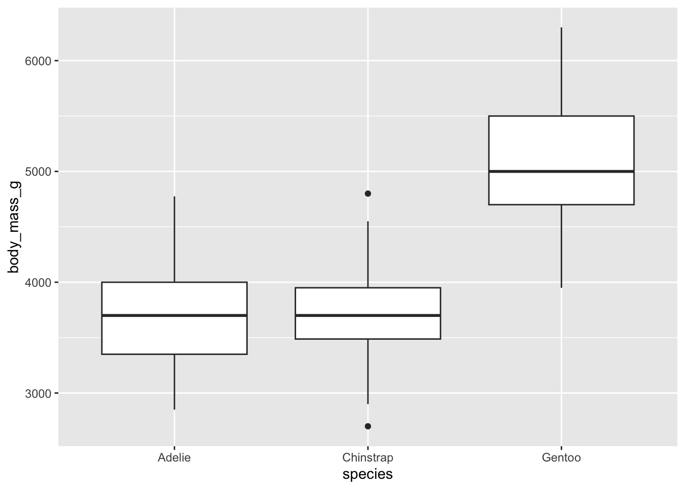
adding labels to the ggplot
Adding more things to the ggplot is a matter of adding additional
+ objects to the plot. We can add labels using the
labs() object. Like boxplot, this allows us to add custom
labels to the x and y axes. We can also add a
title, subtitle, and caption!
# add a geom_boxplot
ggplot(penguins, aes(x = species, y = body_mass_g)) +
geom_boxplot() +
labs(x = 'Species', y = 'Body Mass (g)', title = 'Penguin Body Mass!', subtitle = 'measured in grams', caption = 'whiskers represent interquartile range * 1.5') ## Warning: Removed 2 rows containing non-finite outside the scale range
## (`stat_boxplot()`).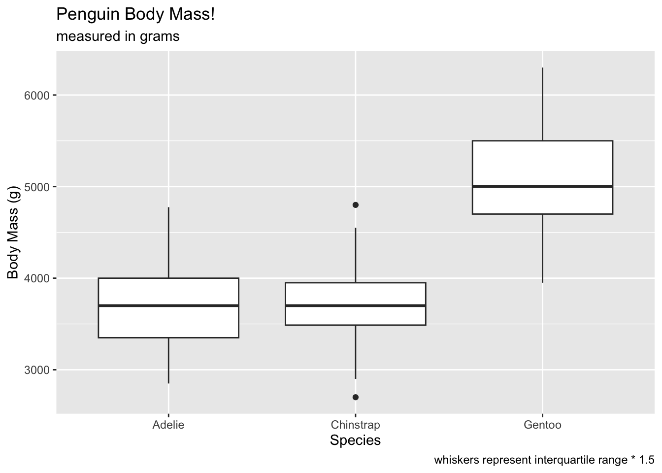
controlling the geom_boxplot()
There are several ways to increase the inferential value of the boxplots.
notchcreates notches around the medians, which can be used to compare whether medians significantly overlap or not. The idea is that notches that overlap suggest no differences between groups:
ggplot(penguins, aes(x = species, y = body_mass_g)) +
  geom_boxplot(notch = T) +
  labs(x = 'Species', y = 'Body Mass (g)', title = 'Penguin Body Mass!', subtitle = 'measured in grams', caption = 'whiskers represent interquartile range * 1.5')
## Warning: Removed 2 rows containing non-finite outside the scale range
## (`stat_boxplot()`).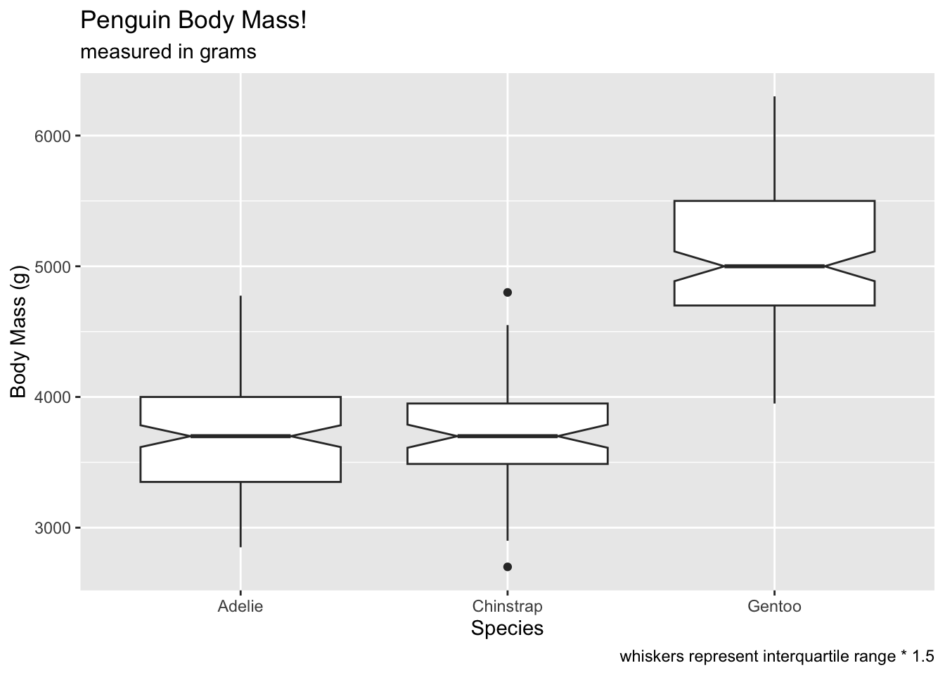
We can also control the length of the whiskers using the
coef argument. This determines how long the whiskers
extend, which is by default 1.5 * the interquartile range.
What happens if we set coef to 1? The number of
“outliers” increases (because the whiskers are shorter). This should be
a good lesson on being careful about letting default settings guide your
interpretations.
ggplot(penguins, aes(x = species, y = body_mass_g)) +
  geom_boxplot(notch = T, coef = 1) +
  labs(x = 'Species', y = 'Body Mass (g)', title = 'Penguin Body Mass!', subtitle = 'measured in grams', caption = 'whiskers represent interquartile range * 1')
## Warning: Removed 2 rows containing non-finite outside the scale range
## (`stat_boxplot()`).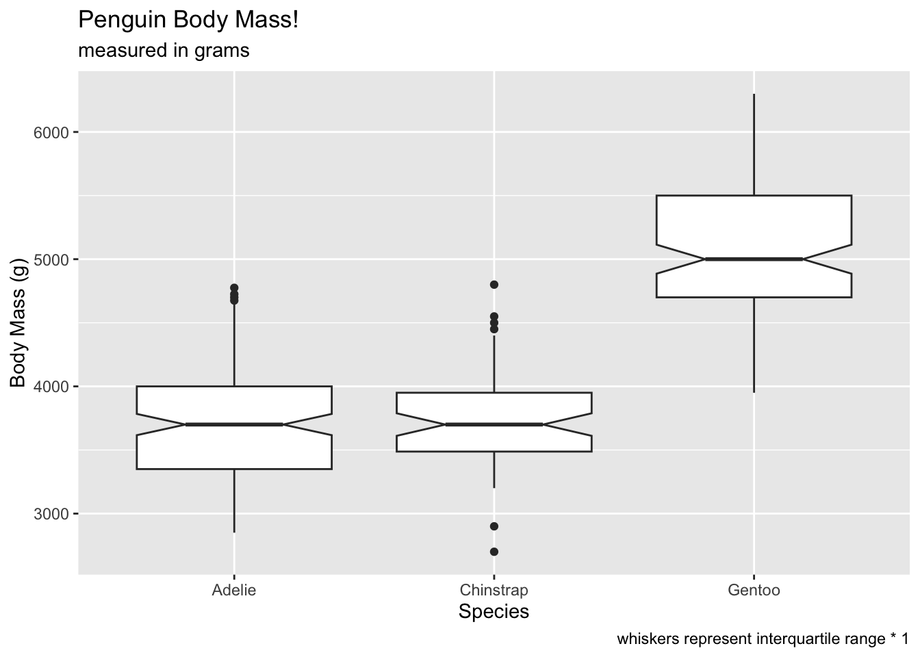
Compare coef at 2…
# voila! no outliers!

ggplot(penguins, aes(x = species, y = body_mass_g)) +
  geom_boxplot(notch = T, coef = 2) +
  labs(x = 'Species', y = 'Body Mass (g)', title = 'Penguin Body Mass!', subtitle = 'measured in grams', caption = 'whiskers represent interquartile range * 2')
## Warning: Removed 2 rows containing non-finite outside the scale range
## (`stat_boxplot()`).
Compare coef at 0.25…
# oops, all outliers.
ggplot(penguins, aes(x = species, y = body_mass_g)) +
  geom_boxplot(notch = T, coef = 0.25) +
  labs(x = 'Species', y = 'Body Mass (g)', title = 'Penguin Body Mass!', subtitle = 'measured in grams', caption = 'whiskers represent interquartile range * 0.25')
## Warning: Removed 2 rows containing non-finite outside the scale range
## (`stat_boxplot()`).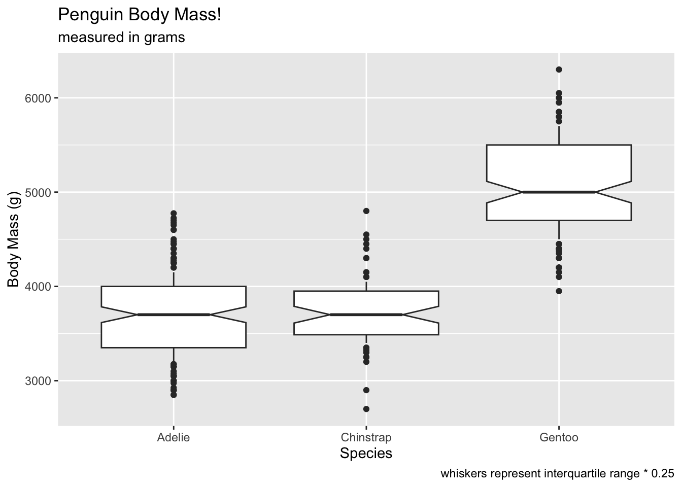
We can set the varwidth argument to TRUE,
which will show the width of the boxplots relative to the total size of
the sample. We can see that chinstrap penguins have a more narrow box
when compared to the Adelie and Gentoo:
# width of boxplots proportional to sqrt(n())
ggplot(penguins, aes(x = species, y = body_mass_g)) +
  geom_boxplot(notch = T, varwidth = T) +
  labs(x = 'Species', y = 'Body Mass (g)', title = 'Penguin Body Mass!', subtitle = 'measured in grams', caption = 'boxplot width reflects n')
## Warning: Removed 2 rows containing non-finite outside the scale range
## (`stat_boxplot()`).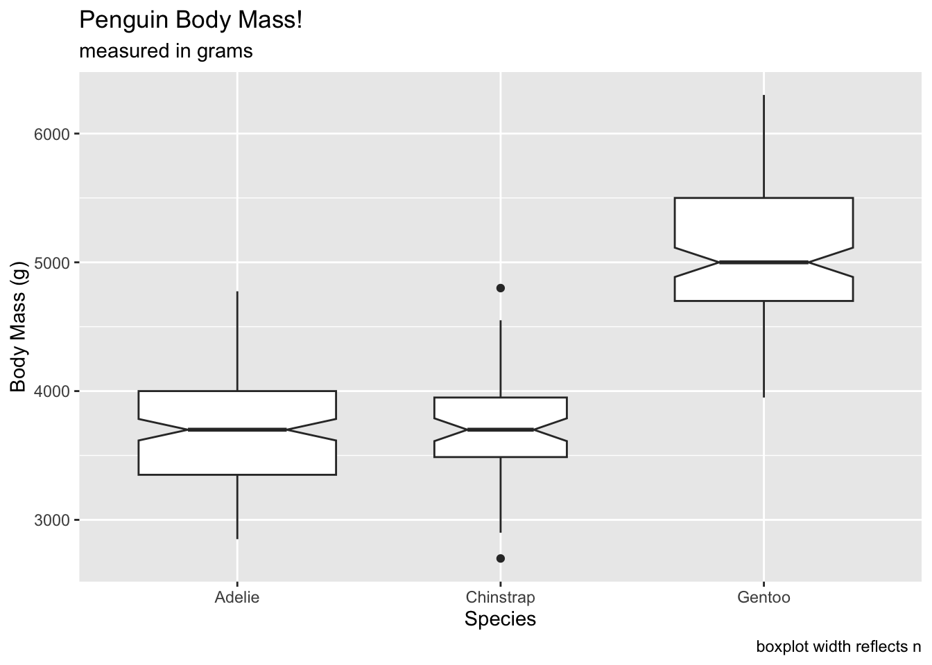
styling the boxplots
If you like the whiskers, you can use staplewidth to get
the whiskers back:
# gimme me whiskers
ggplot(penguins, aes(x = species, y = body_mass_g)) +
  geom_boxplot(notch = T, staplewidth = .5) +
  labs(x = 'Species', y = 'Body Mass (g)', title = 'Penguin Body Mass!', subtitle = 'measured in grams', caption = 'whiskers represent interquartile range * 1.5')
## Warning: Removed 2 rows containing non-finite outside the scale range
## (`stat_boxplot()`).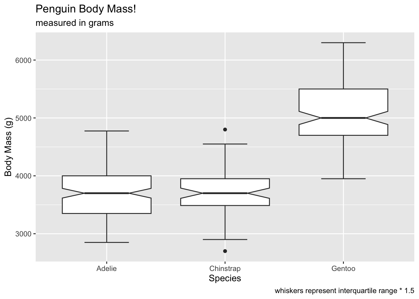
You can choose a colour for the “outliers”
# colour ALL the outliers (bad IQR calculation)
ggplot(penguins, aes(x = species, y = body_mass_g)) +
  geom_boxplot(notch = T, staplewidth = .5, coef = 0, outlier.colour = 'blue')  +
  labs(caption = 'interquartile range * 0')
## Warning: Removed 2 rows containing non-finite outside the scale range
## (`stat_boxplot()`).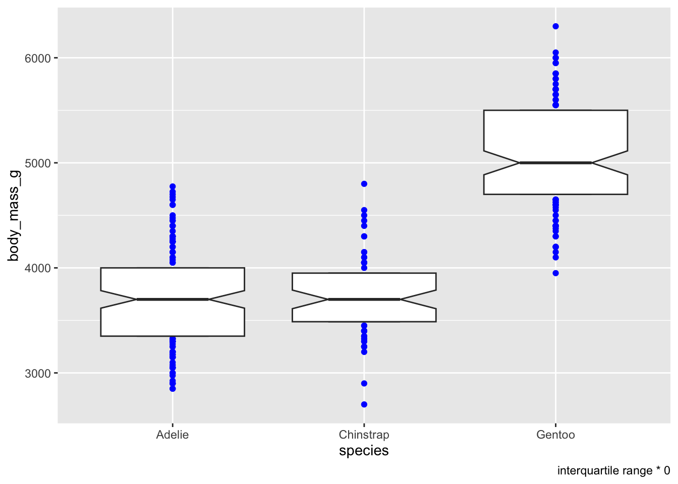
Adding colour to our boxplots:
colorwill add color to the lines/outlines/outliersfillwill control the color inside the boxplots
# use just colour to fill in the boxplots
ggplot(penguins, aes(x = species, y = body_mass_g)) +
  geom_boxplot(notch = T, staplewidth = .5, color = 'lightcoral', fill = 'black')
## Warning: Removed 2 rows containing non-finite outside the scale range
## (`stat_boxplot()`).
Just like col(), we can supply color and
fill with a vector of colours we want to use. The length of
the vectors need to match the number of levels in the group (here, there
are three species, so we supply three colours).
# use just colour to fill in the boxplots
ggplot(penguins, aes(x = species, y = body_mass_g)) +
  geom_boxplot(notch = T, staplewidth = .5,
               color = c('lightcoral', 'dodgerblue', 'green'),
               fill = c('green', 'lightcoral','dodgerblue'))
## Warning: Removed 2 rows containing non-finite outside the scale range
## (`stat_boxplot()`).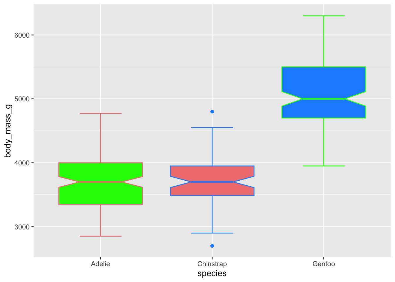
Control the transparency with alpha, which ranges from 0
(transparent) to 1 (opaque)
# use just colour to fill in the boxplots
ggplot(penguins, aes(x = species, y = body_mass_g)) +
  geom_boxplot(notch = T, staplewidth = .5,
               color = c('lightcoral', 'dodgerblue', 'green'),
               fill = c('green', 'lightcoral','dodgerblue'),
               alpha = .5)
## Warning: Removed 2 rows containing non-finite outside the scale range
## (`stat_boxplot()`).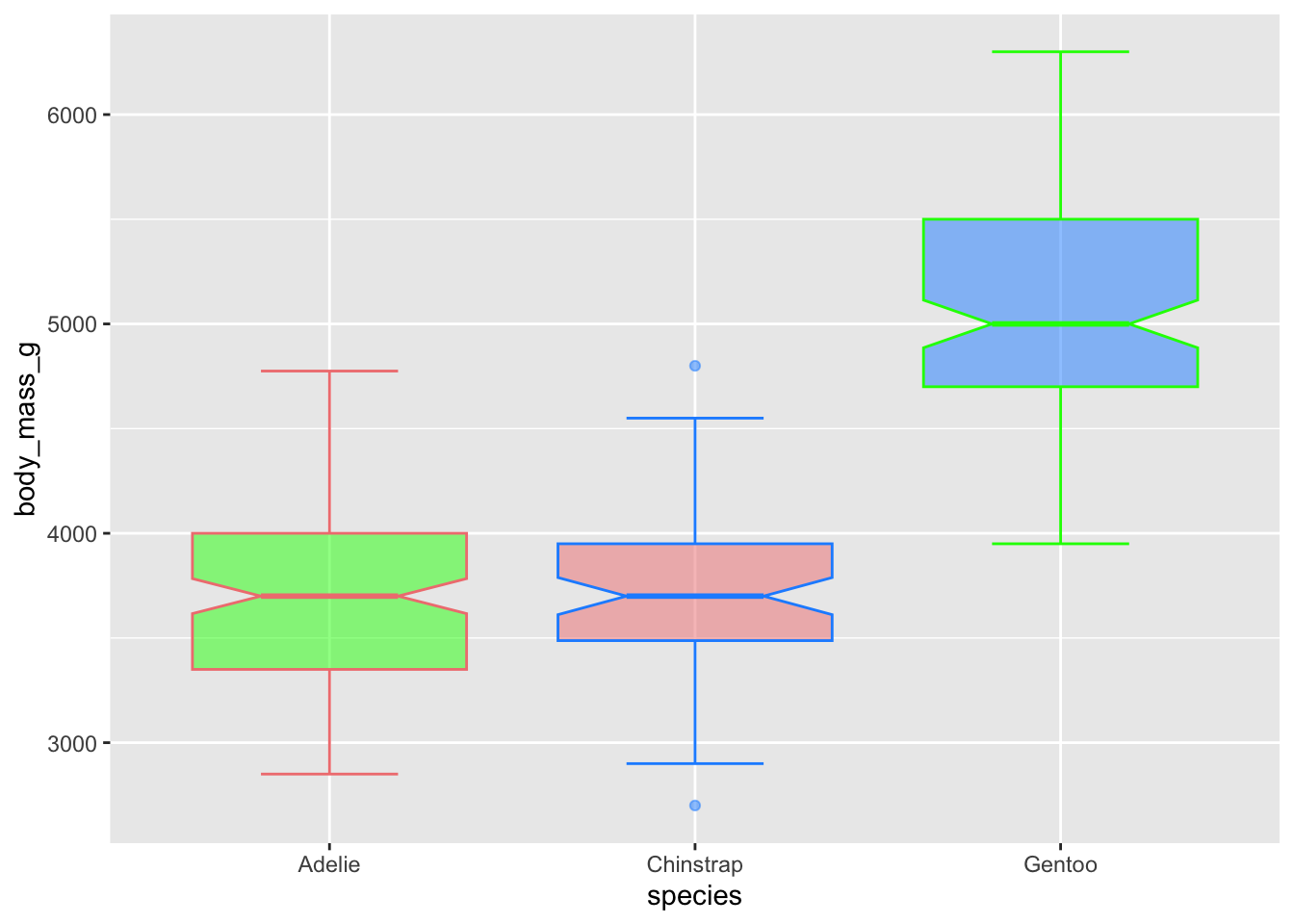
styling within aes()
One of the great things about ggplot is being able to
set many of the aesthetic things within the aes call, and
being able to do this by group.
For example, if we move the fill argument inside the
aes call, we can tell ggplot to fill any relevant geom
based on levels of a grouping variable.
Look at how nice this looks! we also get a spiffy legend!
# use fill in the aes call to fill in the boxplots:
ggplot(penguins, aes(x = species, y = body_mass_g, fill = species)) +
  geom_boxplot()
## Warning: Removed 2 rows containing non-finite outside the scale range
## (`stat_boxplot()`).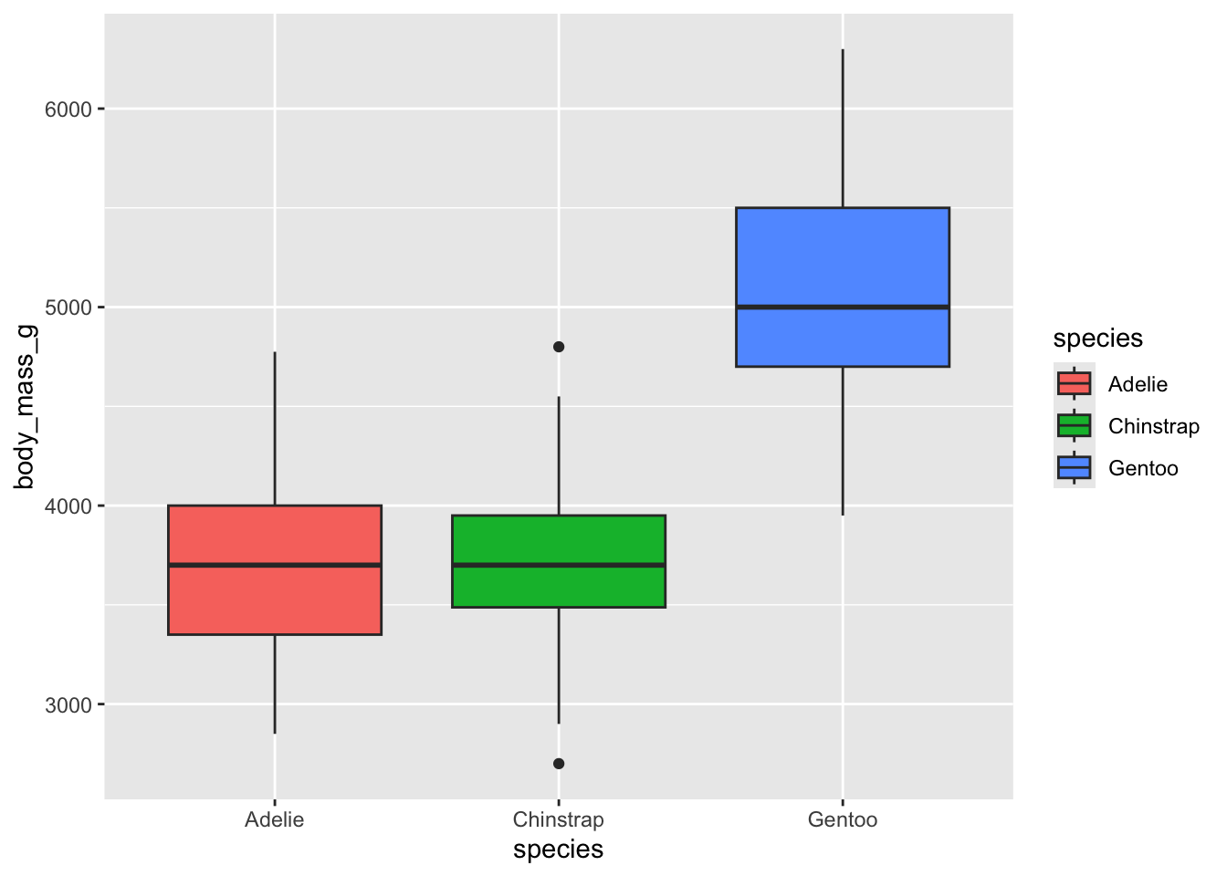
Try putting linetype in the aes call, also set to
species
# adding linetype will add this additional information:
ggplot(penguins, aes(x = species, y = body_mass_g, fill = species, linetype = species)) +
  geom_boxplot(notch = T) +
  # remove x label by giving it an empty string
  labs(y = "Body Mass (g)", x = "")
## Warning: Removed 2 rows containing non-finite outside the scale range
## (`stat_boxplot()`).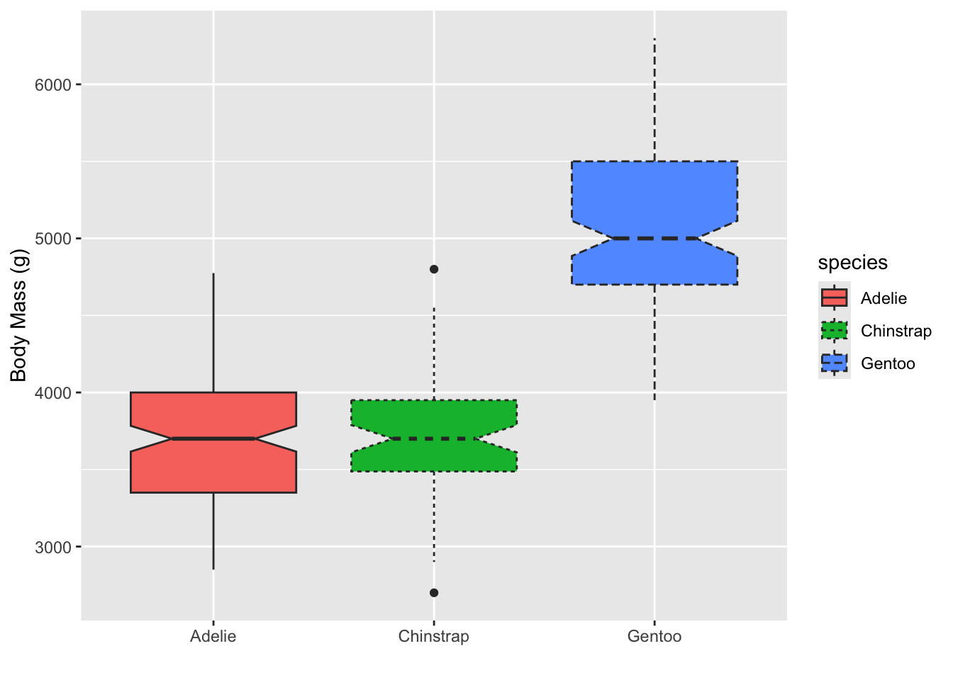
your turn
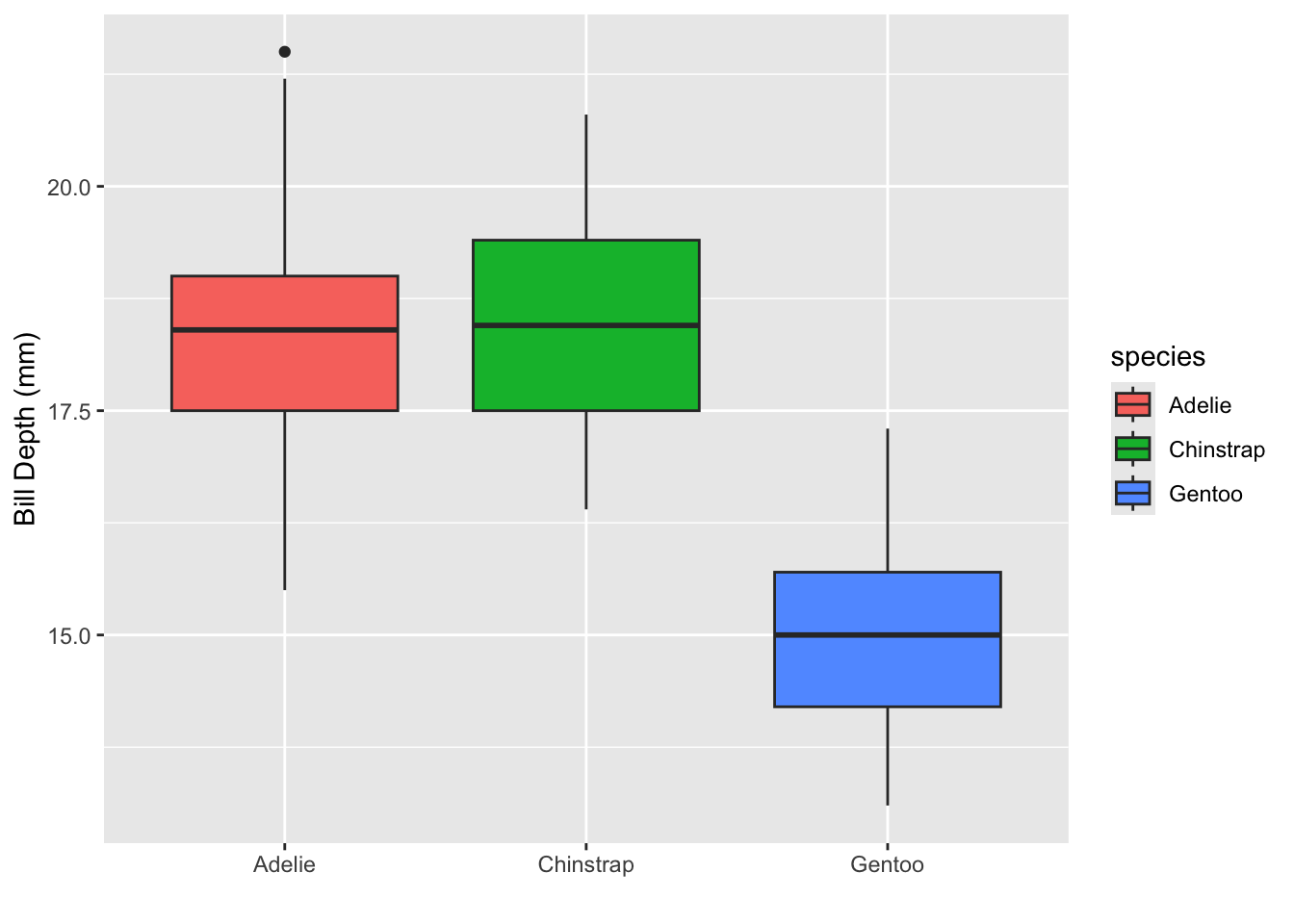
Can you recreate the following plot?
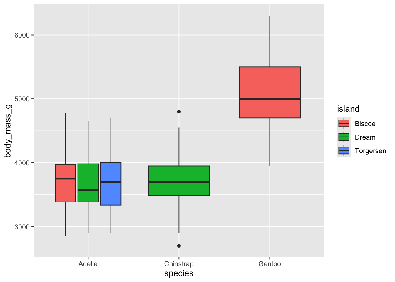
Can you recreate the following plot? You’ll have to think about what
to put inside the fill argument.
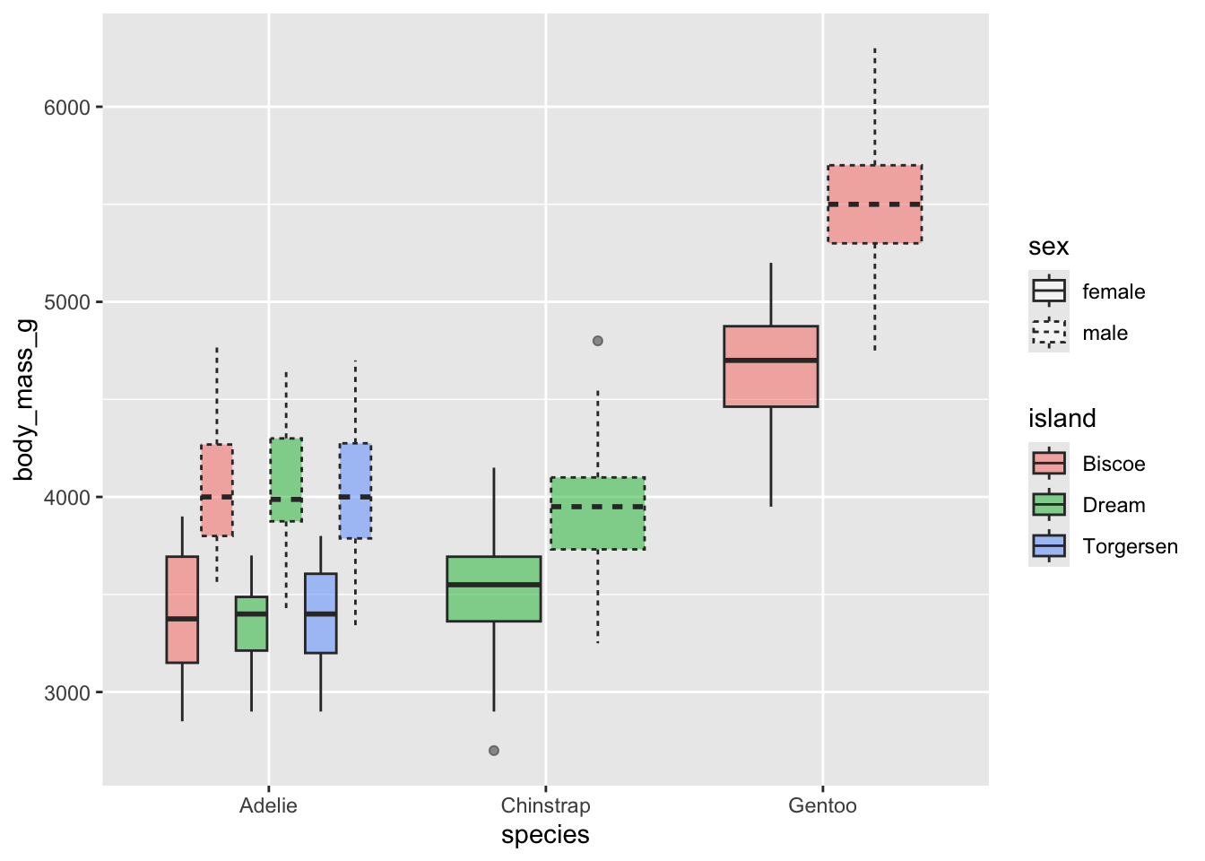
What about this plot? You will need to somehow get rid of
the NA values - can you do it within the ggplot call? The function
drop_na() might be useful.