linear-model
2025-04-10
Without any other information, if you had to guess the weight of a randomly sampled penguin, what would you guess?
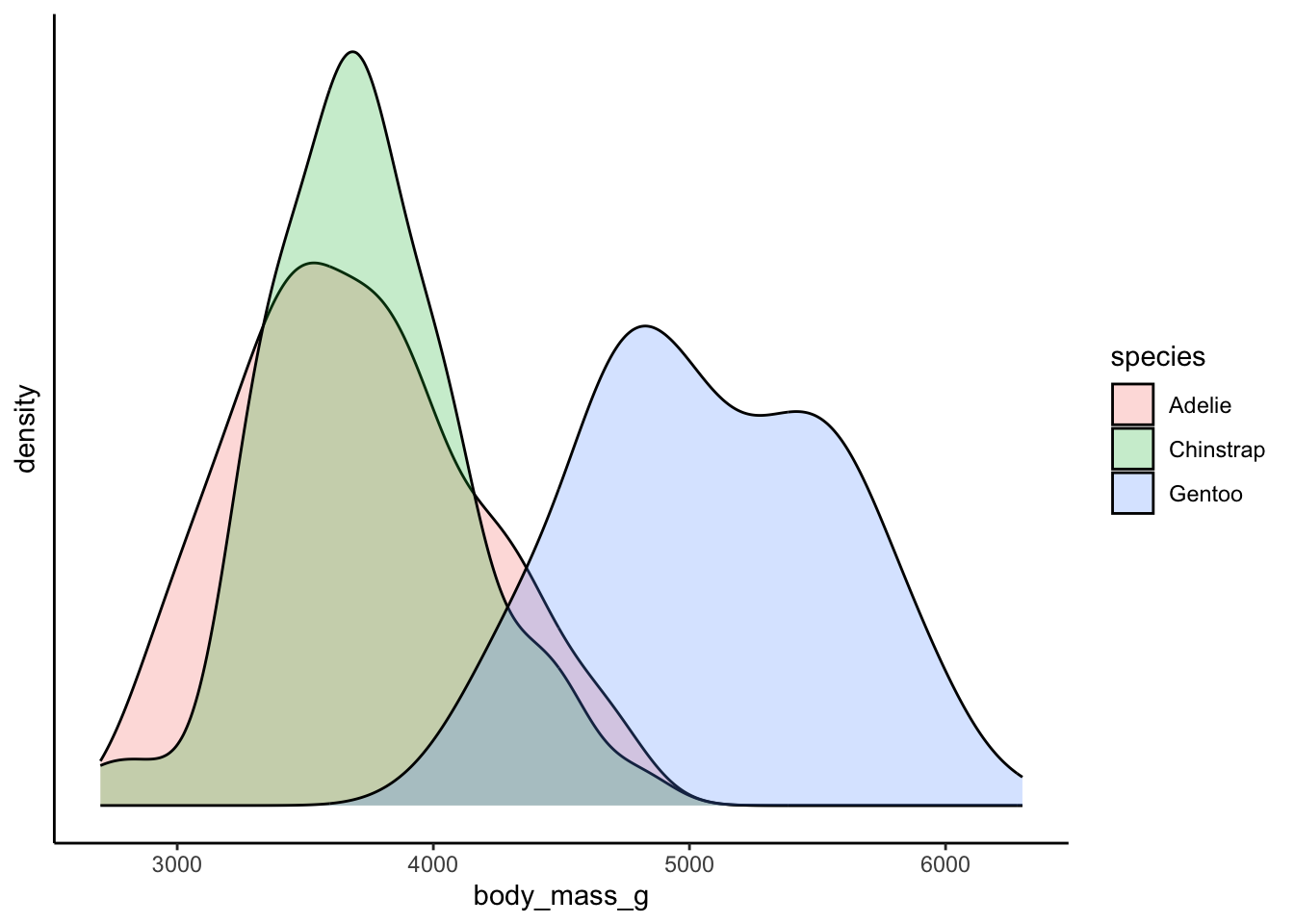
Recall that the mean value of a measure in a population can be used as a prediction.
## [1] 4201.754We might wonder - is it a very good prediction? How good does the mean model perform? And, how good does the mean model perform once we provide it with further information? These questions are essentially what we are asking when we start to perform linear regression or use linear models. Basically, we want to know how well extra information can be used to provide “better” means, or means that vary in response to new information (aka, other variables).
Basic components of a linear model
One way to think about this is whether the mean values can be better
explained as a function of some predictor variable. We want to test the
relationship of our outcome variable in the presence of a predictor
variable. The outcome variable is normally depicted as y,
and the predictor variables are depicted as x. The
y variable is thus our dependent variable. The relationship
between the two, with y varying as a function of
x, can be depicted mathematically as:
\[
\Large y \sim x
\] Think about this in terms of the plots we’ve created, which
have a y-axis and an x-axis. A linear regression is going to provide
information about the y and the x in the form
of a line or a solution defining the relationship between the two. The
linear model will provide a line: where do we start on
y, and where do we end up on x? This is the
basic logic of the intercept and slope
that is provided by linear models.
- The
intercept= starting position fory - The
slope= the magnitude of the effect ofxony.
Consider the scatter plot of penguin body mass:
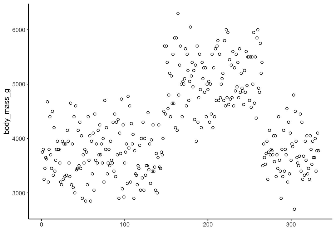
The mean value of penguin body mass is 4201.754386
So without any other information, the
intercept of a linear model for penguin body mass will
be the mean. Because there is no x predictor(s), there will
be a slope of 0. It would look like this:
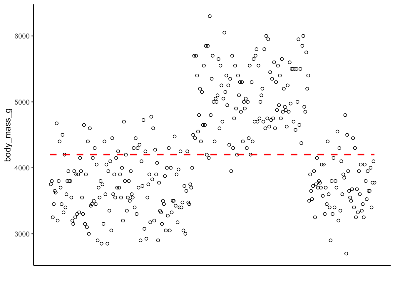
How many points are along the line? How many are close to the line? How many are far away? The relative distance between the points and this intercept represent the predictive ability of the model. The difference between the actual value and the intercept form the residuals of the model. Smaller residuals mean the model did a better job predicting the actual data, whereas larger residuals mean the model is struggling to predict the data points.
fitting a linear model with only the mean
We can fit a linear model with the mean as the only information to
demonstrate this. The basic function for linear model in R is
lm(). The syntax is:
lm(y ~ x, data = ...)But we don’t have an x variable yet! In order to fit an intercept
only model, we can use a 1 on the right-hand side of the
~:
lm(y ~ 1, data = ...)So to fit an intercept-only linear model for penguin body mass, we type this. Note what the output gives you - a reminder of the formula for the linear model that you typed, and then information about the Coefficients. Here we only have one coefficient, the Intercept.
##
## Call:
## lm(formula = body_mass_g ~ 1, data = penguins)
##
## Coefficients:
## (Intercept)
##        4202
We should save the model to a variable:
The summary() function provides us with even more
information about our model:
We again have the call, followed by a description of the distribution of the residuals, followed by the coefficients which now include the standard error, the t value, and a p value, and then some final information about the model. What does this output say?
Well, it is telling us that the predicted value of penguin body mass is 4201.75 grams, which is also the mean of penguin body mass. Light bulb! The starting point for this linear model is the mean of the outcome variable!
##
## Call:
## lm(formula = body_mass_g ~ 1, data = penguins)
##
## Residuals:
##     Min      1Q  Median      3Q     Max
## -1501.8  -651.8  -151.8   548.2  2098.2
##
## Coefficients:
##             Estimate Std. Error t value Pr(>|t|)
## (Intercept)  4201.75      43.36   96.89   <2e-16 ***
## ---
## Signif. codes:  0 '***' 0.001 '**' 0.01 '*' 0.05 '.' 0.1 ' ' 1
##
## Residual standard error: 802 on 341 degrees of freedom
##   (2 observations deleted due to missingness)
looking at the residuals
Recall that the residuals are the differences between the actual values and the model predictions. We can see the residuals from our intercept only model here. Note that the y-axis is now expressed in terms of the distance from the mean. This plot is exactly the same as our raw data, just expressed on a different scale. Think about this - we have effectively performed a linear transformation - subtracting the mean from all of the raw values!

adding an x / predictor variable
Time to add a predictor or independent variable which we think might
help us provide better predictions about penguin body mass. There are
several other body measurements in the data. Let’s look at
flipper_length_mm as a predictor of penguin body weight. We
can think about this in terms of the formula: body mass is the
y, and flipper length is the x
So we are going to condition the mean of body mass within the context of flipper length.
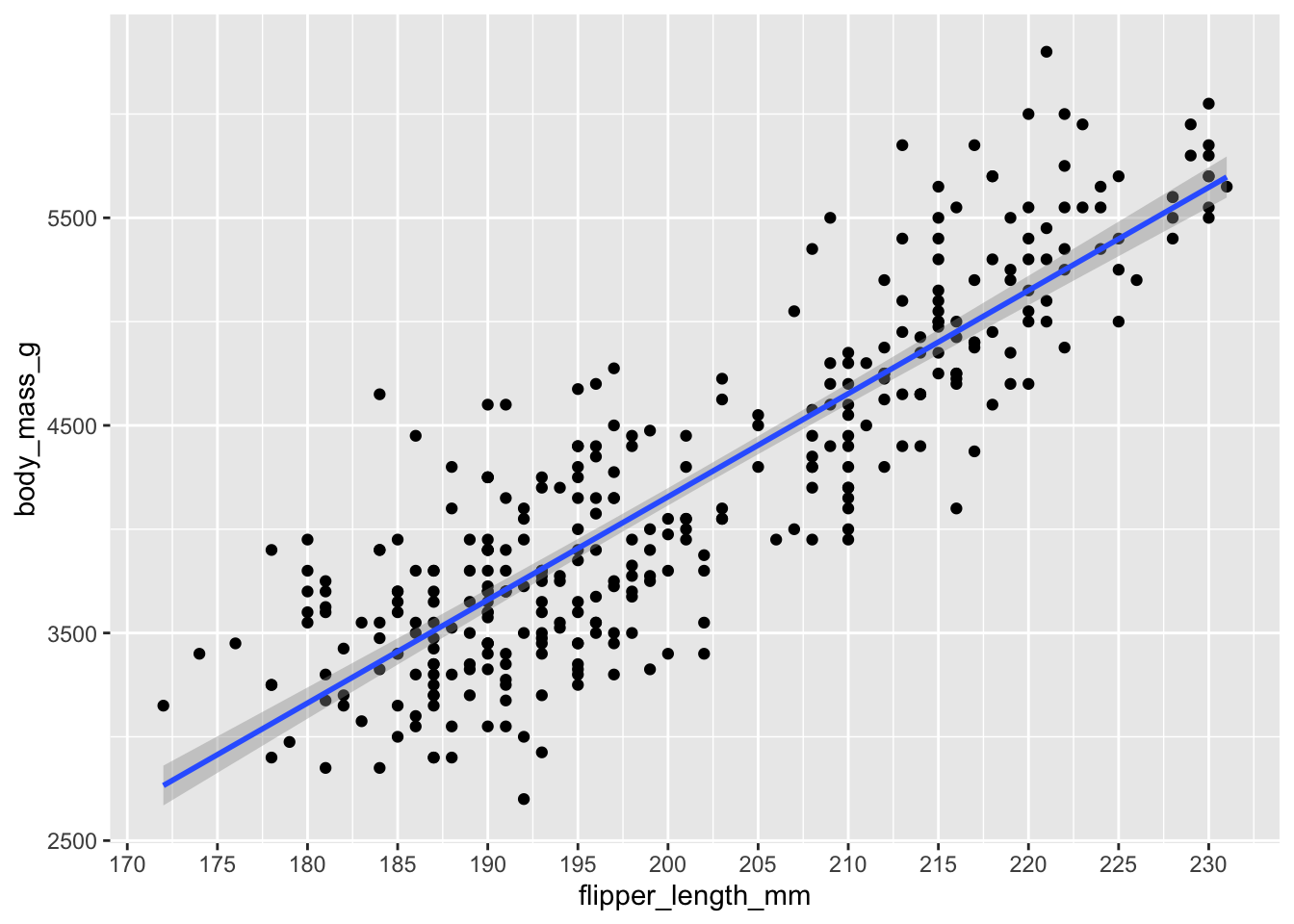
\[ \text{Body Mass} \sim \text{Flipper Length} \] We can plot this relationship before fitting any models. Look at how values of body mass change as flipper length increases - this suggests that flipper length has a linear relationship with body mass. As one thing goes up, the other thing goes up (and sometimes down!). If we plug this into a linear model, we can specify the nature of this relationship in terms of precise units - how much does body mass change for a one-unit increase in flipper length?
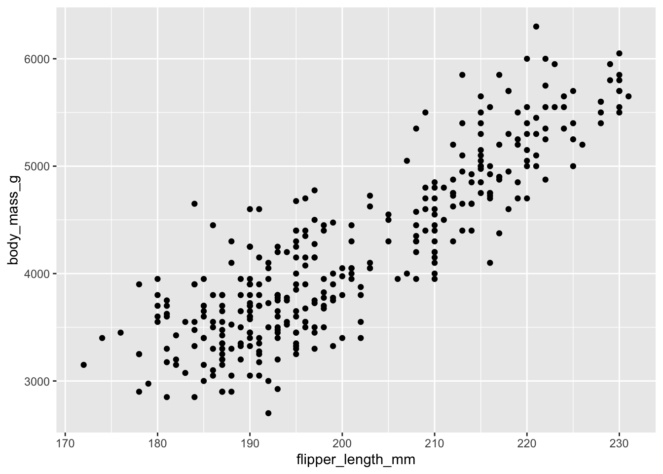
Let us fit the model:
Use the summary to see the model specifications - what is different?
There is new information - we now have information about the role of the predictor variable (flipper length), and also more information about the model itself, in terms of r squared, adjusted r squared, and a F statistic with degrees of freedom and a p value.
Let’s focus on the coefficients of the model for now.
We have a new value for the intercept of about -5780. We also have a
new entry for our x variable:
flipper_length_mm. The estimate for this value is 49.686.
This value is also called the coefficient or the (un-standardized) beta
value.
How do we interpret these values?
Firstly, the new value for the intercept is quite different than the intercept value in the intercept only model! Recall that in the intercept only model, the intercept was the mean (~4201 grams). Here our intercept is a larger absolute value, but is also negative! This is because the default behavior of the linear model is to provide an average for the outcome variable when the predictor variable is equal to zero.
So the interpretation of this regression model is that starting at
-5780 grams, each one-unit increase in flipper length will increase body
mass by 49.686 grams. Because the raw units of
flipper_length_mm are in millimeters, the interpretation
becomes “for each millimeter increase in flipper length, body mass
increases by about 50 grams.”
##
## Call:
## lm(formula = body_mass_g ~ flipper_length_mm, data = penguins)
##
## Residuals:
##      Min       1Q   Median       3Q      Max
## -1058.80  -259.27   -26.88   247.33  1288.69
##
## Coefficients:
##                    Estimate Std. Error t value Pr(>|t|)
## (Intercept)       -5780.831    305.815  -18.90   <2e-16 ***
## flipper_length_mm    49.686      1.518   32.72   <2e-16 ***
## ---
## Signif. codes:  0 '***' 0.001 '**' 0.01 '*' 0.05 '.' 0.1 ' ' 1
##
## Residual standard error: 394.3 on 340 degrees of freedom
##   (2 observations deleted due to missingness)
## Multiple R-squared:  0.759,  Adjusted R-squared:  0.7583
## F-statistic:  1071 on 1 and 340 DF,  p-value: < 2.2e-16
We can express this relationship mathematically:
\[ \text{body weight} = \text{intercept} + \text{coefficient}* x \] The actual formula looks something more like this. The \(\epsilon\) represents the error in the model - the fact that the predictor variable will not be able to perfectly explain the outcome variable. The error comes from the residuals - the distance between the predicted and actual values in the data.
\[
y_i = b_0 + b_1 x_i + \epsilon_i
\] Where:
- \(y_i\) is the dependent variable for
the \(i\)-th observation.
- \(b_0\) is the intercept.
- \(b_1\) is the slope (coefficient of
the predictor).
- \(x_i\) is the predictor variable for
the \(i\)-th observation.
- \(\epsilon_i\) is the error
term.
We can rewrite this formula with the existing information about our
model
\[ \text{body weight} = -5780 + (50 * \text{flipper length}) \]
Let us pretend that we find a new penguin who has a flipper length of 200 millimeters. We can simply plug this value into our regression formula and derive a predicted weight:
\[ \text{body weight} = -5780 + (50 * \text{200}) \]
\[ \text{body weight} = -5780 + 10000 \]
\[ -5780 + 10000 = 4220 \]
Our model thus predicts that if we find a penguin with a flipper that is 200 millimeters long, the body weight will be 4220 grams. This is the basic logic of how to interpret the relationship between the intercept and coefficient(s) of a regression model using a continuous outcome variable.
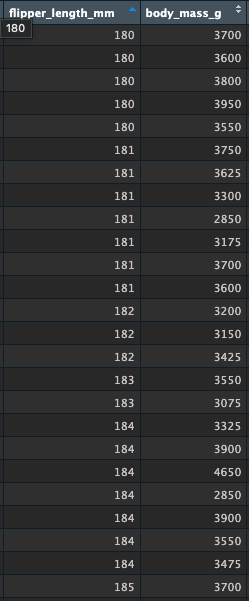
Let’s quickly look at the raw values to see if this makes sense. Here are some values around 200mm of flipper length. How accurate is the predicted value of 4220grams body mass? You can see some variation here, which helps us understand that the model is making predictions about these variables based on the entire distributions, and that these predictions have an inherent level of error:

inspecting the residuals
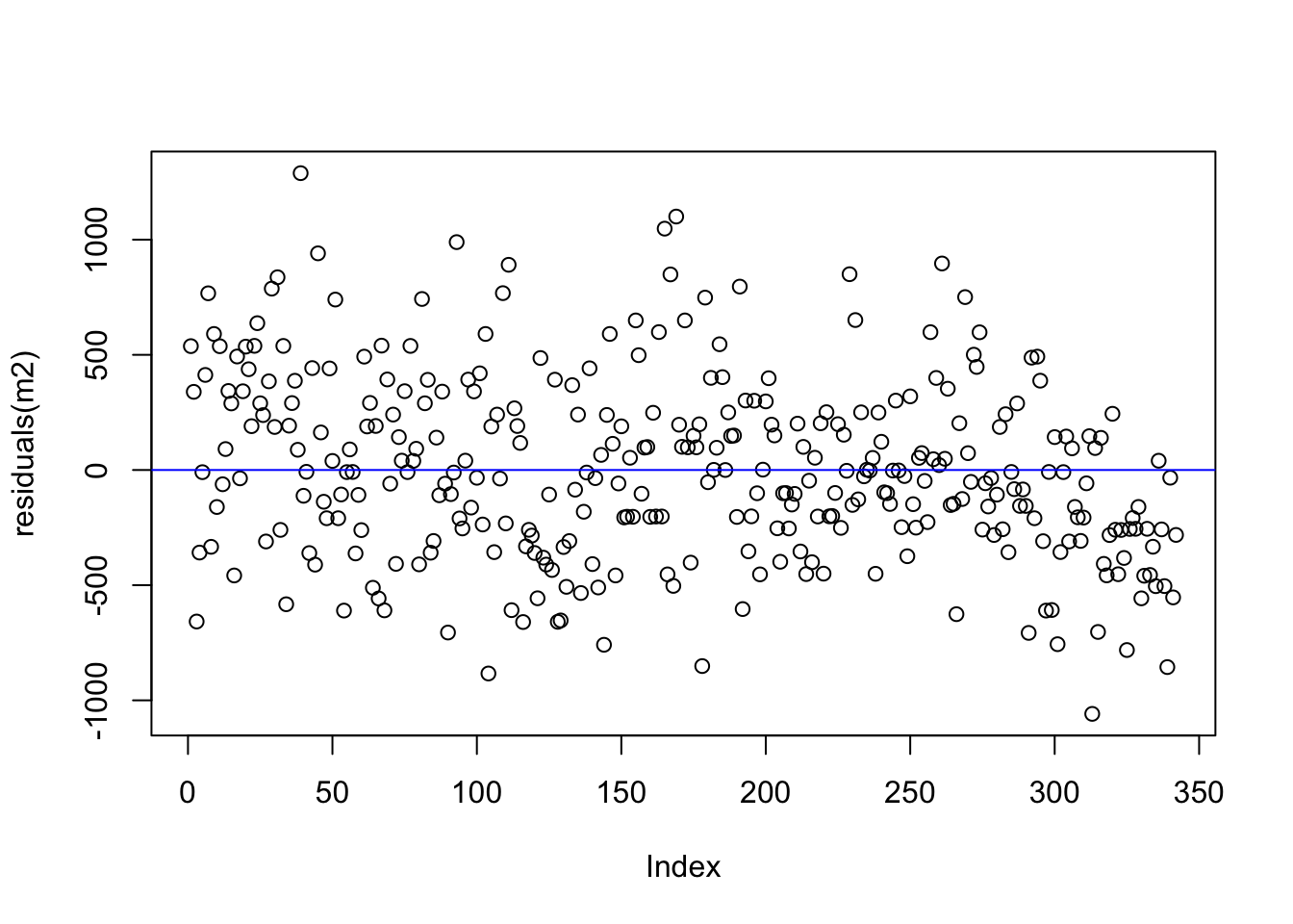
Let’s compare the residuals from the intercept-only model and the model with flipper length as a predictor. Recall that any residual of 0 means that the model was able to almost perfectly predict the actual value.
Compare the spread of the points from zero in both plots - how are they similar/different?
intercept only
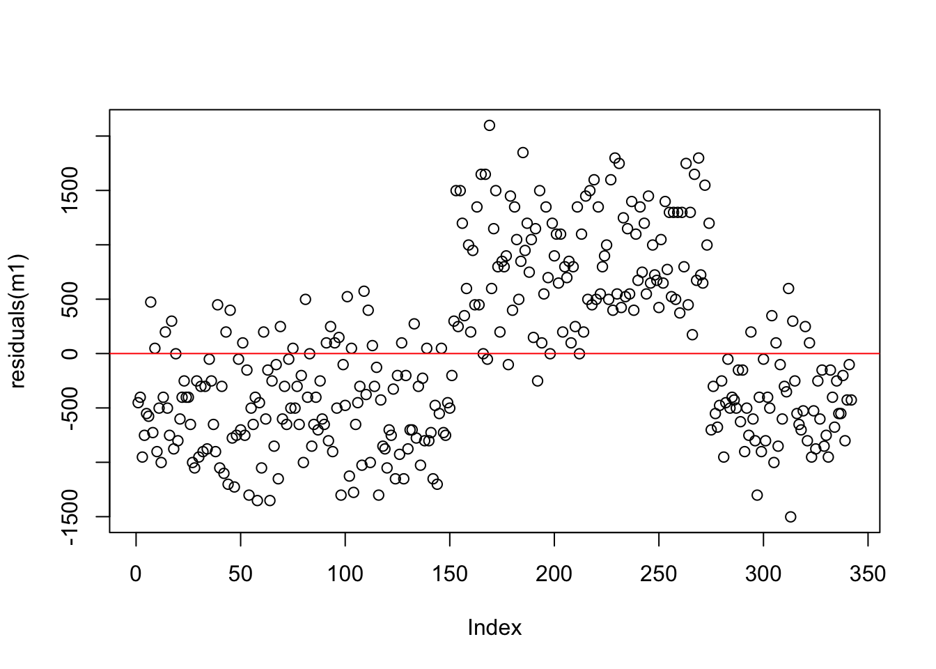
We can see that the residuals for the flipper length model are more uniform in terms of their spread from 0 when compared to the intercept only model. This is some indication of a better model (but there are better ways to assess this).
flipper length predictor
back to those assumptions
There are important assumptions about regression models which relate to the nature of the data. One assumption is that the variance among the residuals is homogeneous which means that the relative distance from zero equally spread out among all the observations. The residual plot above shows us evidence of such homogeneity.
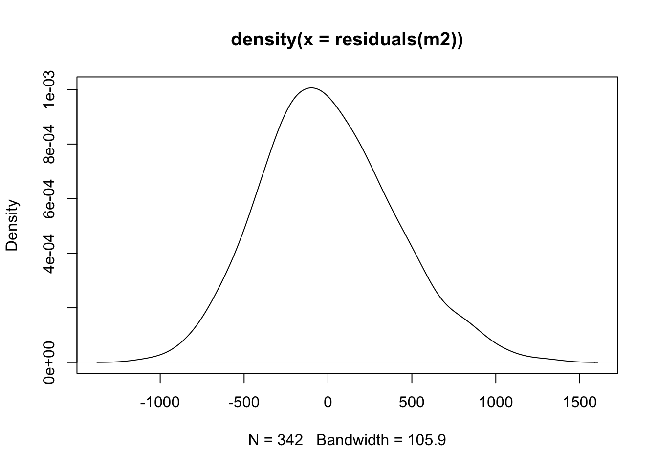
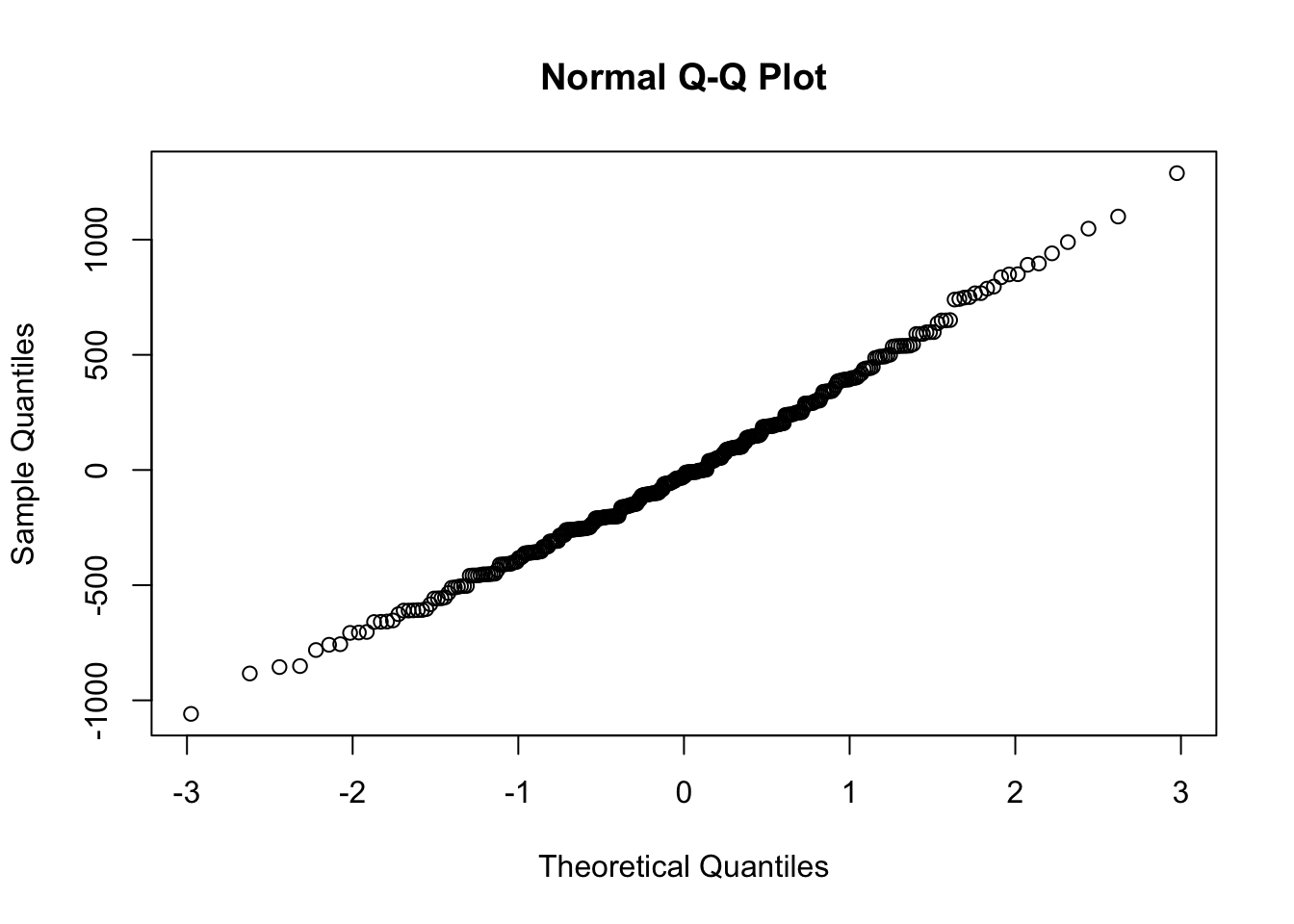
The other is an assumption of normality! What does this assumption relate to? It relates to the distribution of the residuals. The residuals are assumed to follow a normal distribution, and all resulting statistical information follows this assumption. This means that the standard errors, confidence intervals, test statistics, and p-values are all derived under the assumption that the error in the model is normally distributed.
Take a look at a density plot of the residuals - does this resemble a normal distribution?
A qqplot (quantile-quantile) will sample the residuals along different assumed portions of a normal distribution. If the residuals follow a normal distribution, they will line up as a straight line:
Model predictions versus reality
Let’s wrap up by connecting this model to a previous lesson on the effects of centering predictor variables.
Recall that when we center, we subtract each value by the mean of that value, like so:
# create a new variable which is centered flipper length (in millimeters)
penguins$flipper_length_mm_c <- penguins$flipper_length_mm - mean(penguins$flipper_length_mm, na.rm = T)
The linear transformation means that the new variable has a mean of zero, and the values represent each value’s distance from that mean:
##    Min. 1st Qu.  Median    Mean 3rd Qu.    Max.    NA's
## -28.915 -10.915  -3.915   0.000  12.085  30.085       2
Fit a new model with the centered predictor variable:
Call the summary - what has changed?
Remember, the intercept will provide us with the predicted value of the outcome variable when the predictor variable is held at zero. Since the mean flipper length is now zero, our intercept shows us the mean value of body mass when flipper length is held at its mean as well.
What does this do to the intercept? It resets it to the mean of body mass! We now have an intercept that is plausible.
What about the effect of flipper length on body mass? The estimate is the exact same as it was in the version where the variable was not centered. This should make intuitive sense when we remember that a linear transformation does not change the overall distribution of a variable - it merely slides the variable along the distribution.
So what is the point of centering in this case? It provides us with a better interpretation of the model data. Now we can say that each one-unit increase from the mean of flipper length results in an increase of 50grams from the mean of body mass. Moreover, it is impossible for a penguin to have a flipper length of 0mm, so we are also interpreting that scale in a more meaningful way
(please also note how nothing related to significance has changed - linear transformations of predictors do not change their distributions, so this will not change their overall relationship with other variables as well. )
##
## Call:
## lm(formula = body_mass_g ~ flipper_length_mm_c, data = penguins)
##
## Residuals:
##      Min       1Q   Median       3Q      Max
## -1058.80  -259.27   -26.88   247.33  1288.69
##
## Coefficients:
##                     Estimate Std. Error t value Pr(>|t|)
## (Intercept)         4201.754     21.320  197.08   <2e-16 ***
## flipper_length_mm_c   49.686      1.518   32.72   <2e-16 ***
## ---
## Signif. codes:  0 '***' 0.001 '**' 0.01 '*' 0.05 '.' 0.1 ' ' 1
##
## Residual standard error: 394.3 on 340 degrees of freedom
##   (2 observations deleted due to missingness)
## Multiple R-squared:  0.759,  Adjusted R-squared:  0.7583
## F-statistic:  1071 on 1 and 340 DF,  p-value: < 2.2e-16
We can write the new formula like this to make new predictions, but we have to be careful and center our value first! Here is how we can write it out:
\[ \text{body mass} = 4201 + (50 * (\text{flipper length} - \text{mean}(\text{flipper length})) \]
A reminder of the mean value of flipper length:
## [1] 200.9152Let’s just say the mean is 200 for simplicity. Apply this prediction to our a new penguin with a flipper length of 180 mm:
\[ \text{body mass} = 4201 + (50 * (180-200) \] \[ \text{body mass} = 4201 + (50 * -20) \] And here is our predicted body weight for a penguin with a flipper length of 180mm:
\[ 4201 + -1000 = 3181 \]
Look again at the data around this flipper length:
visualise a one-predictor lm()
We can use ggplot() to visualize this one-predictor
regression model using the geom_smooth() geom. We add
method = 'lm' to tell the geom to use a linear model.
The degree of the line is the slope - how much does y
change for a one-unit increase in x? The answer is 50
grams!
ggplot(penguins, aes(y = body_mass_g, x = flipper_length_mm)) +
  geom_point() +
  geom_smooth(method = 'lm')
## `geom_smooth()` using formula = 'y ~ x'## Warning: Removed 2 rows containing non-finite outside the scale range
## (`stat_smooth()`).## Warning: Removed 2 rows containing missing values or values outside the scale
## range (`geom_point()`).
We can force the x-axis to show us more precise values in 5mm intervals. Compare the y-axis between any two points. Because they differ by 5mm, the y axis should change by about 250g (the slope is ~50, so 50 * 5 = 250).
This is essentially what the output of the linear model is telling us.
ggplot(penguins, aes(y = body_mass_g, x = flipper_length_mm)) +
  geom_point() +
  geom_smooth(method = 'lm') +
  scale_x_continuous(breaks = seq(from = 170, to = 230, by = 5))