categorical by categorical
Stephen Skalicky
2024-12-04
In this notebook we will consider a third type of interaction - categorical by categorical. We will further complicate this by using a two level * three level categorical interaction.
We will ask the question is there an interaction between penguin species and sex on body mass?
Before moving on, please consider what this interaction is asking. Recall that an interaction is a conditional effect, meaning that the effect of one variable depends on another.
# load libraries
library(tidyverse)
library(palmerpenguins)
library(emmeans)
data(penguins)
penguins <- drop_na(penguins)
We already know that sex has a significant “effect” on body weight, as we’ve already explored it before. The default dummy coding scheme. Here we see that, on average, penguin males are 683 grams heavier than penguin females.
##
## Call:
## lm(formula = body_mass_g ~ sex, data = penguins)
##
## Residuals:
##     Min      1Q  Median      3Q     Max
## -1295.7  -595.7  -237.3   737.7  1754.3
##
## Coefficients:
##             Estimate Std. Error t value Pr(>|t|)
## (Intercept)  3862.27      56.83  67.963  < 2e-16 ***
## sexmale       683.41      80.01   8.542  4.9e-16 ***
## ---
## Signif. codes:  0 '***' 0.001 '**' 0.01 '*' 0.05 '.' 0.1 ' ' 1
##
## Residual standard error: 730 on 331 degrees of freedom
## Multiple R-squared:  0.1806, Adjusted R-squared:  0.1781
## F-statistic: 72.96 on 1 and 331 DF,  p-value: 4.897e-16
Look at the effects of species
Then what does an interaction ask for? It will ask whether this male-female difference depends on or is conditional on penguin species.
Now let’s look at species, which is a three-level categorical variable
## [1] "Adelie" "Chinstrap" "Gentoo"We can see the number of cases per level:
##    Adelie Chinstrap    Gentoo
##       146        68       119
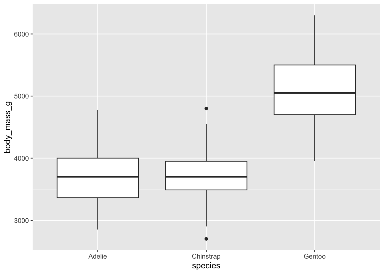
We have some evidence that body mass is different among penguin species.

And we can see the way the contrast coding works for dummy variables. What does it mean for both Chinstrap and Gentoo to be coded as 1, with Adelie as 0?
##           Chinstrap Gentoo
## Adelie            0      0
## Chinstrap         1      0
## Gentoo            0      1
Fitting a model may help to demonstrate the effect - note that we have two coefficients, one for Chinstrap, and one for Gentoo. They are both being compared to the baseline level - Adelie. So when compared to Adelia, Chinstrap has a body mass on average 27 grams heavier, and Gentoo have a body mass on average 1386 grams heavier.
##
## Call:
## lm(formula = body_mass_g ~ species, data = penguins)
##
## Residuals:
##      Min       1Q   Median       3Q      Max
## -1142.44  -342.44   -33.09   307.56  1207.56
##
## Coefficients:
##                  Estimate Std. Error t value Pr(>|t|)
## (Intercept)       3706.16      38.14  97.184   <2e-16 ***
## speciesChinstrap    26.92      67.65   0.398    0.691
## speciesGentoo     1386.27      56.91  24.359   <2e-16 ***
## ---
## Signif. codes:  0 '***' 0.001 '**' 0.01 '*' 0.05 '.' 0.1 ' ' 1
##
## Residual standard error: 460.8 on 330 degrees of freedom
## Multiple R-squared:  0.6745, Adjusted R-squared:  0.6725
## F-statistic: 341.9 on 2 and 330 DF,  p-value: < 2.2e-16
What contrast are we missing…? Fortunately we can use another library to get these contrasts, but more on that later. But, look, we can see that the contrast between Adelie and Chinstrap is not significant, whereas the other contrasts are!
## $emmeans
##  species   emmean   SE  df lower.CL upper.CL
##  Adelie      3706 38.1 330     3631     3781
##  Chinstrap   3733 55.9 330     3623     3843
##  Gentoo      5092 42.2 330     5009     5176
##
## Confidence level used: 0.95
##
## $contrasts
##  contrast           estimate   SE  df t.ratio p.value
##  Adelie - Chinstrap    -26.9 67.7 330  -0.398  0.9164
##  Adelie - Gentoo     -1386.3 56.9 330 -24.359  <.0001
##  Chinstrap - Gentoo  -1359.3 70.0 330 -19.406  <.0001
##
## P value adjustment: tukey method for comparing a family of 3 estimates
Let’s look at this with contrast coding, where we now have 3 levels of our variable turned into sum coding. Each column will sum to 0.
Previously, with 2 levels, 0 represented the “midpoint” between the two groups if they were coded as -1 and 1.
Here it is different. The group with a 1 is now compared to the other two groups - note that 0 + -1 = -1. So 0 becomes the “midpoint” between the group coded as 1 and the average of the other two groups.
##           [,1] [,2]
## Adelie       1    0
## Chinstrap    0    1
## Gentoo      -1   -1
With that in mind, can we interpret this regression?
The coefficients go in the same order as the levels of the variable
Species 1 = Adelie Species 2 = Chinstrap
The intercept is the grant mean of all penguins
So species1 is the deviation of Adelie compared to the
mean of Chinstrap + Gentoo
And species2 is the deviation of Chinstrap from the mean
of Adelie + Gentoo
What do we lose/gain with this approach?
##
## Call:
## lm(formula = body_mass_g ~ species, data = penguins)
##
## Residuals:
##      Min       1Q   Median       3Q      Max
## -1142.44  -342.44   -33.09   307.56  1207.56
##
## Coefficients:
##             Estimate Std. Error t value Pr(>|t|)
## (Intercept)  4177.23      26.59  157.12   <2e-16 ***
## species1     -471.07      34.52  -13.65   <2e-16 ***
## species2     -444.14      41.80  -10.62   <2e-16 ***
## ---
## Signif. codes:  0 '***' 0.001 '**' 0.01 '*' 0.05 '.' 0.1 ' ' 1
##
## Residual standard error: 460.8 on 330 degrees of freedom
## Multiple R-squared:  0.6745, Adjusted R-squared:  0.6725
## F-statistic: 341.9 on 2 and 330 DF,  p-value: < 2.2e-16
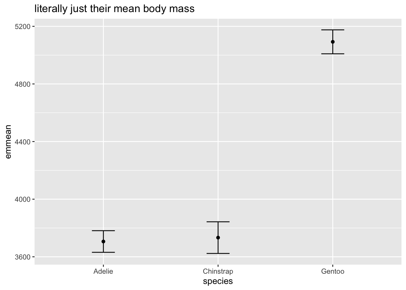
Regardless of coding, when we plot the model predictions, we know we are just getting the mean body mass at these different species:
##  species     emmean       SE  df lower.CL upper.CL
##  Adelie    3706.164 38.13563 330 3631.145 3781.184
##  Chinstrap 3733.088 55.87955 330 3623.163 3843.013
##  Gentoo    5092.437 42.24097 330 5009.341 5175.533
##
## Confidence level used: 0.95ggplot(m3_emmeans, aes(y = emmean, x = species)) +
geom_point() +
geom_errorbar(aes(ymin = lower.CL, ymax = upper.CL),width = .2) +
labs(title = 'literally just their mean body mass')
actually fit the interactions
reset species to dummy coding
##           Chinstrap Gentoo
## Adelie            0      0
## Chinstrap         1      0
## Gentoo            0      1
Now we are getting more complicated.
The interaction here has made things difficult to interpret
The intercept is when species AND sex is at baseline. So the intercept is Adelie, female penguins.
Everything else is being compared to this intercept -
speciesChinstrap is now comparing the difference between
the variable species and the baseline (intercept). This
means it will be female Chinstrap vs. female Adelie. Same thing for
speciesGentoo.
The coefficient sexmale will then be male Adelie
vs. female Adelie (a difference of 674 grams)
The interaction terms then show us how much to adjust the
sexmale effect for the other two levels of species:
The difference between male and female chinstrap is -262 grams less than the difference between male and female Adelie penguins
The difference between male and female Gentoo is 130 grams more than the difference between male and female Adelie penguins
##
## Call:
## lm(formula = body_mass_g ~ species * sex, data = penguins)
##
## Residuals:
##     Min      1Q  Median      3Q     Max
## -827.21 -213.97   11.03  206.51  861.03
##
## Coefficients:
##                          Estimate Std. Error t value Pr(>|t|)
## (Intercept)               3368.84      36.21  93.030  < 2e-16 ***
## speciesChinstrap           158.37      64.24   2.465  0.01420 *
## speciesGentoo             1310.91      54.42  24.088  < 2e-16 ***
## sexmale                    674.66      51.21  13.174  < 2e-16 ***
## speciesChinstrap:sexmale  -262.89      90.85  -2.894  0.00406 **
## speciesGentoo:sexmale      130.44      76.44   1.706  0.08886 .
## ---
## Signif. codes:  0 '***' 0.001 '**' 0.01 '*' 0.05 '.' 0.1 ' ' 1
##
## Residual standard error: 309.4 on 327 degrees of freedom
## Multiple R-squared:  0.8546, Adjusted R-squared:  0.8524
## F-statistic: 384.3 on 5 and 327 DF,  p-value: < 2.2e-16
is my interaction ‘significant?’
There are a variety of ways to test if an interaction is significant, one is the model comparison approach
## Analysis of Variance Table
##
## Model 1: body_mass_g ~ species * sex
## Model 2: body_mass_g ~ species + sex
##   Res.Df      RSS Df Sum of Sq     F    Pr(>F)
## 1    327 31302628
## 2    329 32979185 -2  -1676557 8.757 0.0001973 ***
## ---
## Signif. codes:  0 '***' 0.001 '**' 0.01 '*' 0.05 '.' 0.1 ' ' 1
using emmeans
An invaluable way to decompose a fit model
Emmeans lets us look at estimated marginal means in the model:
## NOTE: Results may be misleading due to involvement in interactions## species emmean SE df lower.CL upper.CL
## Adelie 3706 25.6 327 3656 3757
## Chinstrap 3733 37.5 327 3659 3807
## Gentoo 5082 28.4 327 5026 5138
##
## Results are averaged over the levels of: sex
## Confidence level used: 0.95## NOTE: Results may be misleading due to involvement in interactions## sex emmean SE df lower.CL upper.CL
## female 3859 25.3 327 3809 3908
## male 4489 25.2 327 4440 4539
##
## Results are averaged over the levels of: species
## Confidence level used: 0.95## species sex emmean SE df lower.CL upper.CL
## Adelie female 3369 36.2 327 3298 3440
## Chinstrap female 3527 53.1 327 3423 3632
## Gentoo female 4680 40.6 327 4600 4760
## Adelie male 4043 36.2 327 3972 4115
## Chinstrap male 3939 53.1 327 3835 4043
## Gentoo male 5485 39.6 327 5407 5563
##
## Confidence level used: 0.95The pairwise or pairs functions lets us
make comparisons:
Does this show us the interaction?
## sex = female:
##  contrast           estimate   SE  df t.ratio p.value
##  Adelie - Chinstrap     -158 64.2 327  -2.465  0.0377
##  Adelie - Gentoo       -1311 54.4 327 -24.088  <.0001
##  Chinstrap - Gentoo    -1153 66.8 327 -17.246  <.0001
##
## sex = male:
##  contrast           estimate   SE  df t.ratio p.value
##  Adelie - Chinstrap      105 64.2 327   1.627  0.2357
##  Adelie - Gentoo       -1441 53.7 327 -26.855  <.0001
##  Chinstrap - Gentoo    -1546 66.2 327 -23.345  <.0001
##
## P value adjustment: tukey method for comparing a family of 3 estimates
Does this show us the interaction?
## species = Adelie:
##  contrast      estimate   SE  df t.ratio p.value
##  female - male     -675 51.2 327 -13.174  <.0001
##
## species = Chinstrap:
##  contrast      estimate   SE  df t.ratio p.value
##  female - male     -412 75.0 327  -5.487  <.0001
##
## species = Gentoo:
##  contrast      estimate   SE  df t.ratio p.value
##  female - male     -805 56.7 327 -14.188  <.0001
Do either of those posthocs show us the answer to the interaction: does the effect of sex depend on species?
we still don’t know what is “Significant” about this effect!
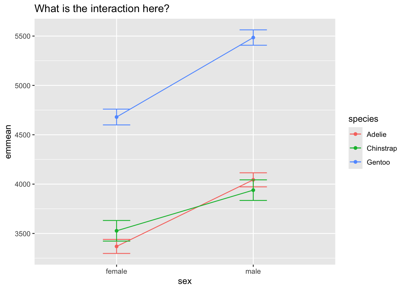
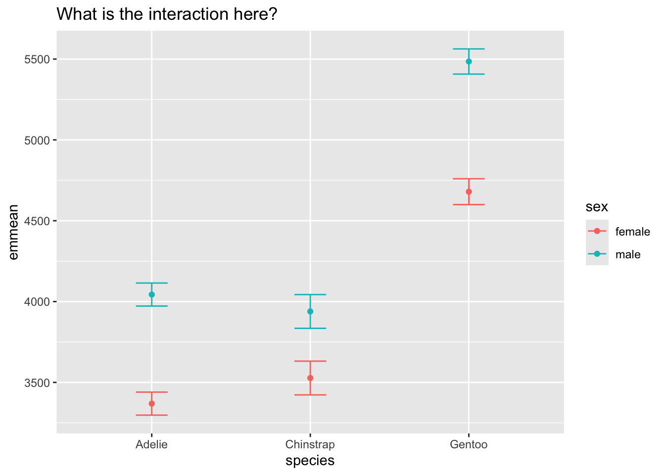
Let’s look at two different plots
dat <- as.data.frame(emmeans(m4, ~ species|sex))

ggplot(dat, aes(y = emmean, x = sex, color = species, group = species)) +
  geom_point() +
  geom_line() +
  geom_errorbar(aes(ymin = lower.CL, ymax = upper.CL), width = .2) +
  labs(title = 'What is the interaction here?')
dat <- as.data.frame(emmeans(m4, ~ species|sex))

ggplot(dat, aes(y = emmean, x = species, color = sex, group = sex)) +
  geom_point() +
  geom_errorbar(aes(ymin = lower.CL, ymax = upper.CL), width = .2)  +
  labs(title = 'What is the interaction here?')
The true reason for the interaction is that the difference between male and female pensguins is stronger for one species when compared to the others. Again, emmeans can show this to us.
Here I ask for the model to show me the differences of differences - and compare them - to find which male/female difference is different/not different among the groups:
Here we see that the difference between female/male is smaller for Chinstrap when compared to Adelie, and larger for Gentoo when compared to Chinstrap
##  species_pairwise   sex_pairwise  estimate   SE  df t.ratio p.value
##  Adelie - Chinstrap female - male     -263 90.8 327  -2.894  0.0041
##  Adelie - Gentoo    female - male      130 76.4 327   1.706  0.0889
##  Chinstrap - Gentoo female - male      393 94.1 327   4.181  <.0001
Note that the summary almost gave us this whole picture:
##
## Call:
## lm(formula = body_mass_g ~ species * sex, data = penguins)
##
## Residuals:
##     Min      1Q  Median      3Q     Max
## -827.21 -213.97   11.03  206.51  861.03
##
## Coefficients:
##                          Estimate Std. Error t value Pr(>|t|)
## (Intercept)               3368.84      36.21  93.030  < 2e-16 ***
## speciesChinstrap           158.37      64.24   2.465  0.01420 *
## speciesGentoo             1310.91      54.42  24.088  < 2e-16 ***
## sexmale                    674.66      51.21  13.174  < 2e-16 ***
## speciesChinstrap:sexmale  -262.89      90.85  -2.894  0.00406 **
## speciesGentoo:sexmale      130.44      76.44   1.706  0.08886 .
## ---
## Signif. codes:  0 '***' 0.001 '**' 0.01 '*' 0.05 '.' 0.1 ' ' 1
##
## Residual standard error: 309.4 on 327 degrees of freedom
## Multiple R-squared:  0.8546, Adjusted R-squared:  0.8524
## F-statistic: 384.3 on 5 and 327 DF,  p-value: < 2.2e-16
This shows us again that trying to interpret the effects without post-hoc modeling may indeed drive us to madness.